Visualizing various types of data
Lecture 3
Duke University
STA 199 - Spring 2024
2024-01-23
Warm up
While you wait…
Questions from the prepare materials?
From last time
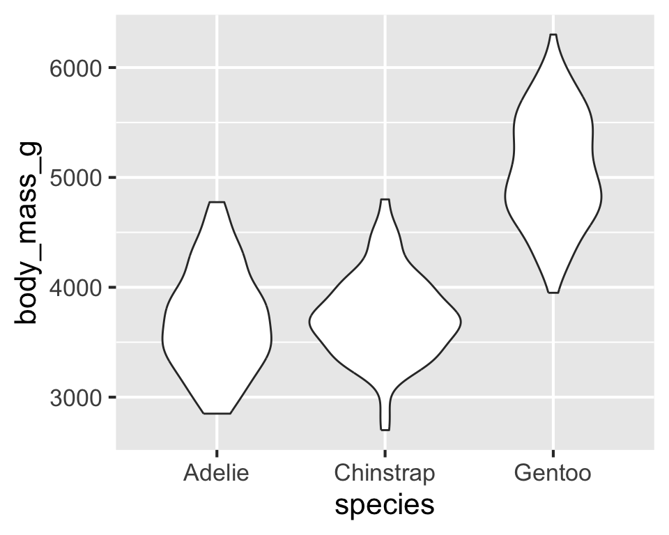
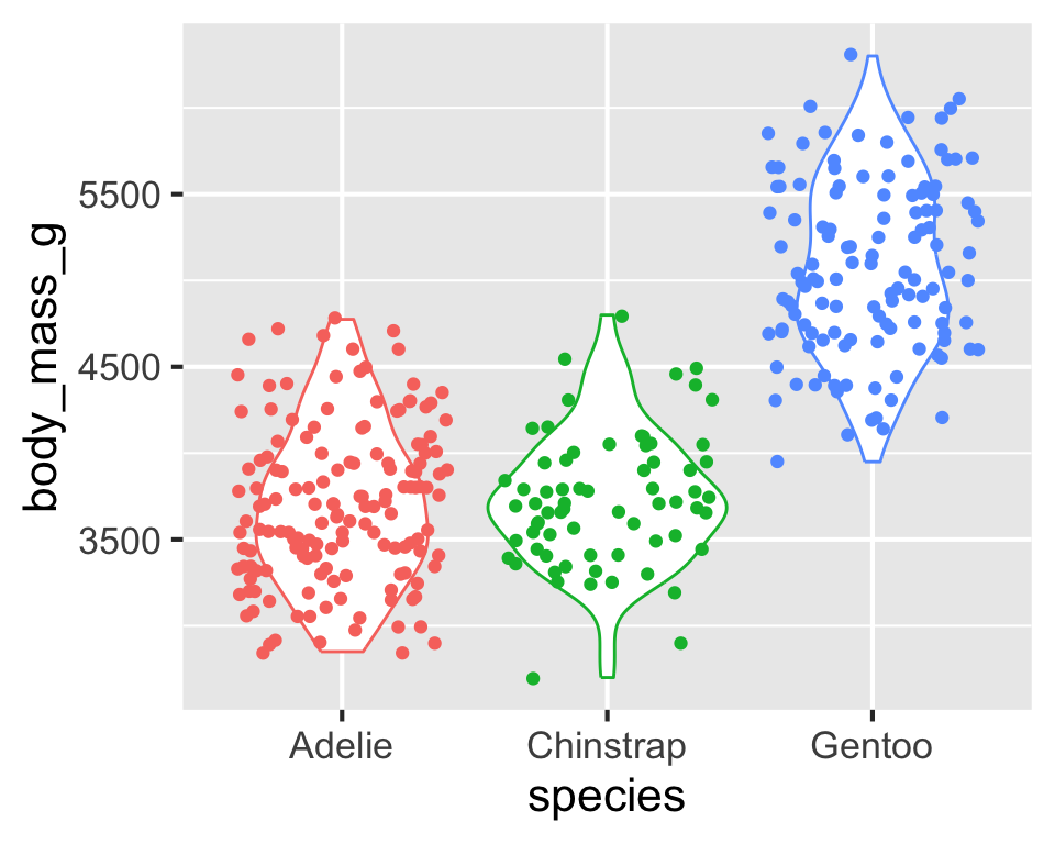
Violin plots
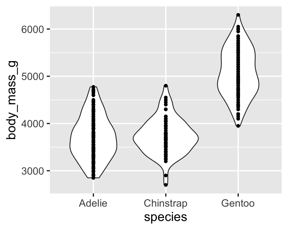
Multiple geoms
Multiple geoms
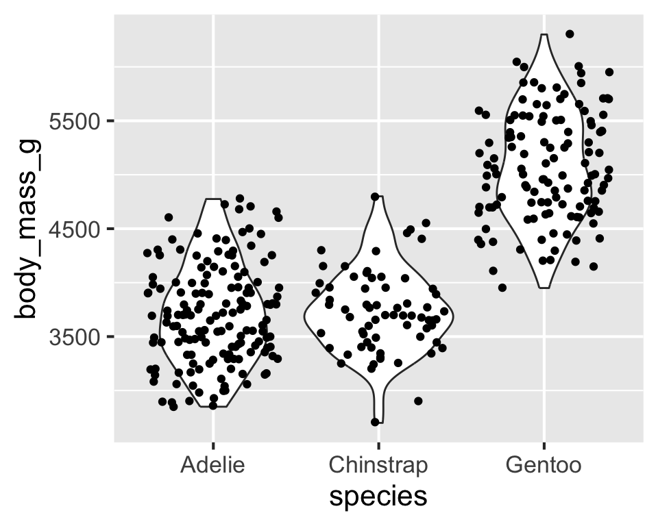
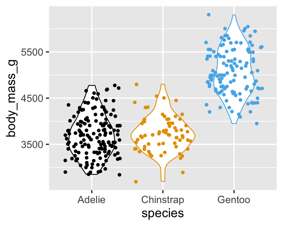
Multiple geoms + aesthetics
Multiple geoms + aesthetics
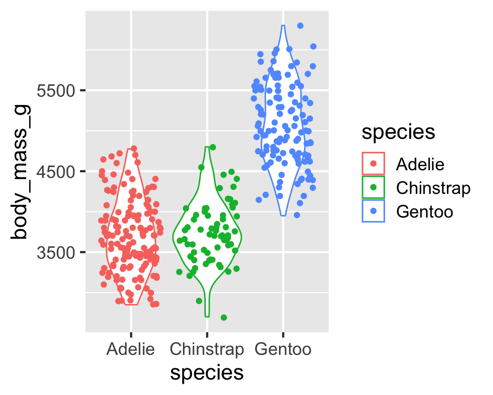
Multiple geoms + aesthetics
Warm up
While you wait…
Questions from the prepare materials?
Questions from last time
Is there any code in the videos that is not in the readings? Yes and no. There is no substantial functionality introduced in the videos that is not also in the readings, however the examples in the videos are different than the ones in the reading.
What are all of the
geoms we need to know? You don’t need to “memorize” or even “know” all o the geoms available in the ggplot2 package, but you can find a list of them on the ggplot2 cheat sheet or on the reference page.Could you please clarify what situations it would be appropriate to use each geom function? Today’s topic! And think about it as “what plot should I make for which type of variable”.
Announcements
- AEs this week should be submitted by midnight on Sunday. To “submit”, commit and push at least once to your
aerepo for each application exercise this week. - If you email me, please put STA 199 in the subject.
From last time
ae-02-bechdel-dataviz
If you were in class last Thursday:
and followed along with the application exercise…
Go to the project navigator in RStudio (top right corner of your RStudio window) and open the project called ae. If there are any uncommitted files, commit them so you can start with a clean slate.
If you missed class last Thursday:
or didn’t follow along with the application exercise…
Go to the course GitHub org and find your ae repo. Clone the repo in your container, open the Quarto document called ae-02-bechdel.
Recap of AE
- Construct plots with
ggplot(). - Layers of ggplots are separated by
+s. - The formula is (almost) always as follows:
- Aesthetic attributes of a geometries (color, size, transparency, etc.) can be mapped to variables in the data or set by the user, e.g.
color = binaryvs.color = "pink". - Use
facet_wrap()when faceting (creating small multiples) by one variable andfacet_grid()when faceting by two variables.
Visualizing various types of data
Identifying variable types
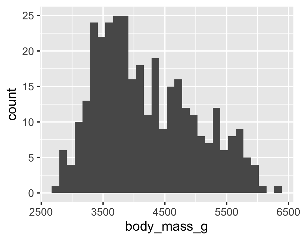
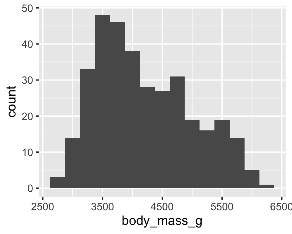
The way data is displayed matters
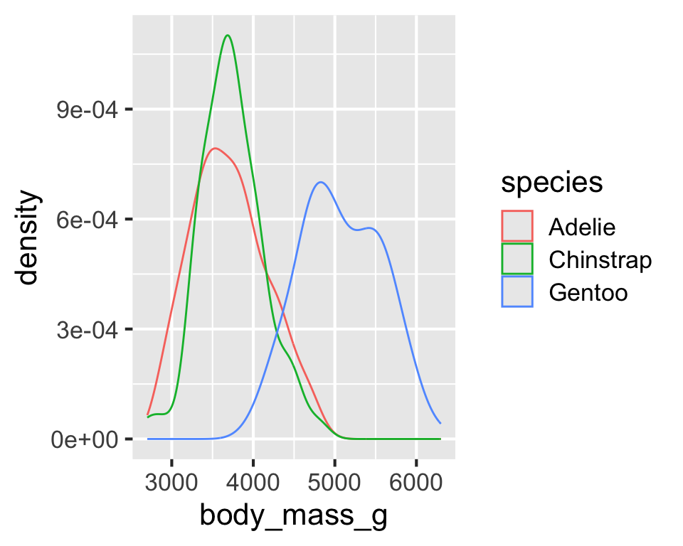
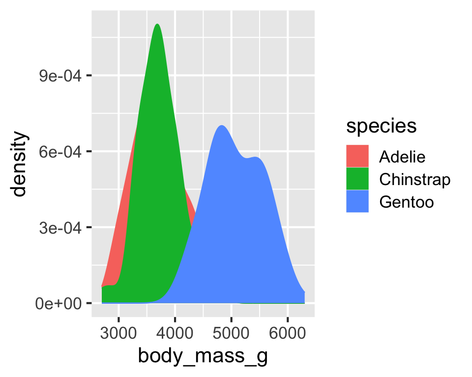
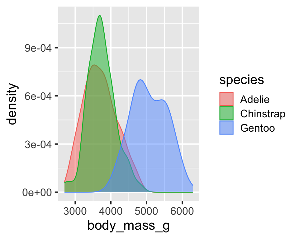
What do these three plots show?

Visualizing penguins
# A tibble: 344 × 8
   species island   bill_length_mm bill_depth_mm flipper_length_mm body_mass_g sex    year
   <fct>   <fct>             <dbl>         <dbl>             <int>       <int> <fct> <int>
 1 Adelie  Torgers…           39.1          18.7               181        3750 male   2007
 2 Adelie  Torgers…           39.5          17.4               186        3800 fema…  2007
 3 Adelie  Torgers…           40.3          18                 195        3250 fema…  2007
 4 Adelie  Torgers…           NA            NA                  NA          NA <NA>   2007
 5 Adelie  Torgers…           36.7          19.3               193        3450 fema…  2007
 6 Adelie  Torgers…           39.3          20.6               190        3650 male   2007
 7 Adelie  Torgers…           38.9          17.8               181        3625 fema…  2007
 8 Adelie  Torgers…           39.2          19.6               195        4675 male   2007
 9 Adelie  Torgers…           34.1          18.1               193        3475 <NA>   2007
10 Adelie  Torgers…           42            20.2               190        4250 <NA>   2007
# ℹ 334 more rows
Univariate analysis
Univariate analysis
Analyzing a single variable:
Numerical: histogram, box plot, density plot, etc.
Categorical: bar plot, pie chart, etc.
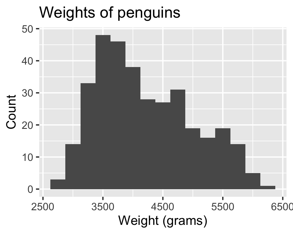
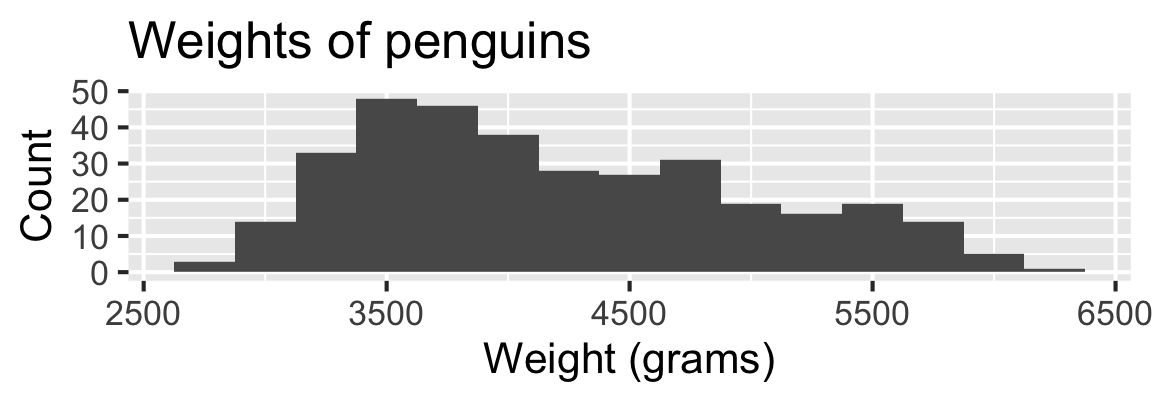
Histogram - Step 1
Histogram - Step 2
Histogram - Step 3
Histogram - Step 4
Histogram - Step 5
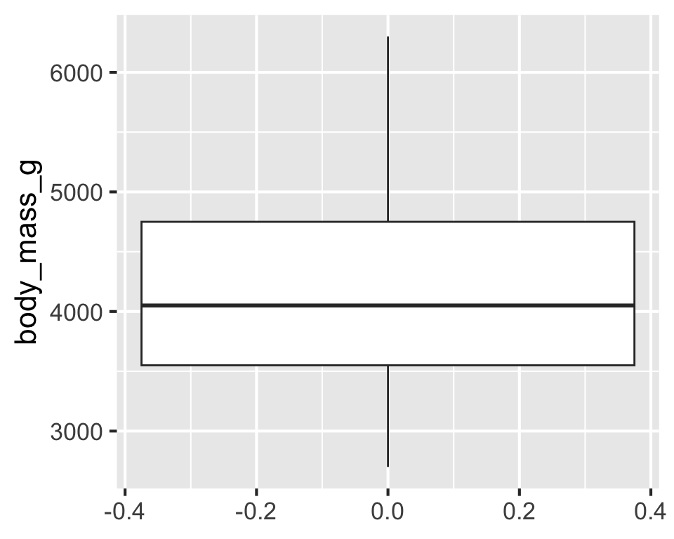
Boxplot - Step 1
Boxplot - Step 2
Boxplot - Step 3
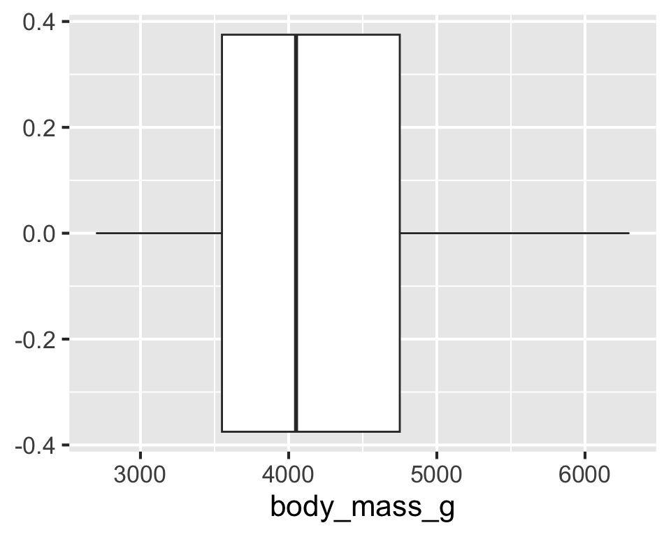
Boxplot - Step 4
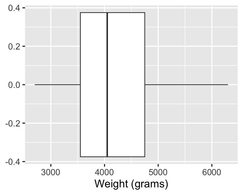
Boxplot - Step 5
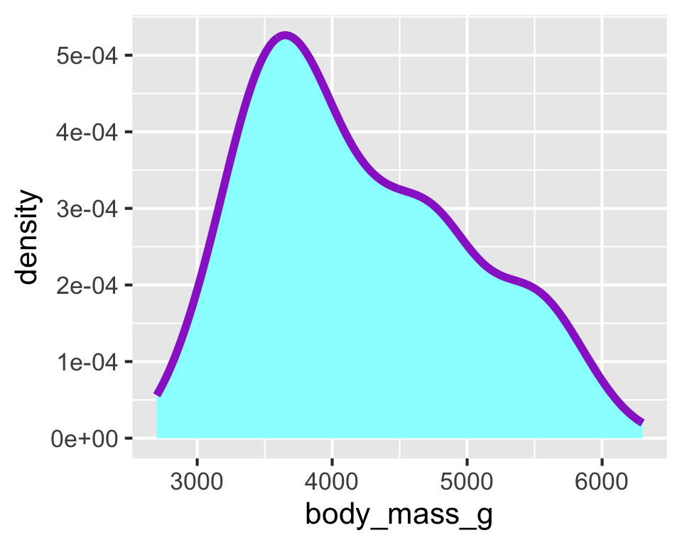
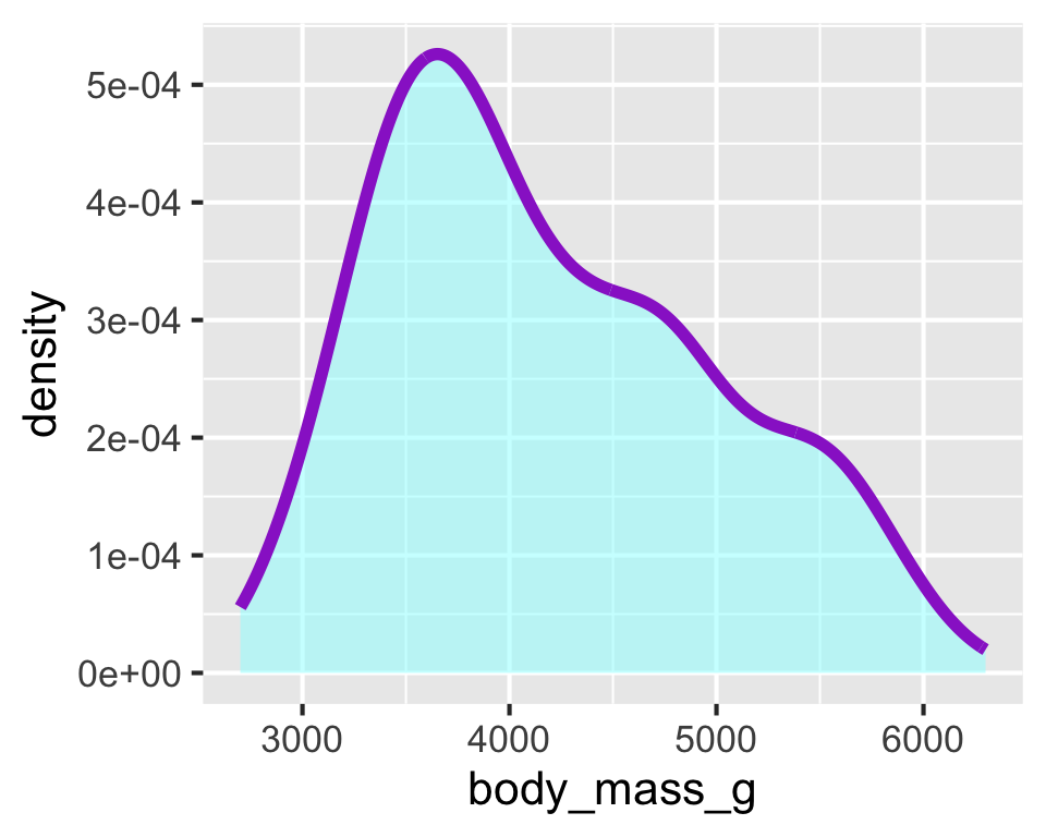
Density plot - Step 1
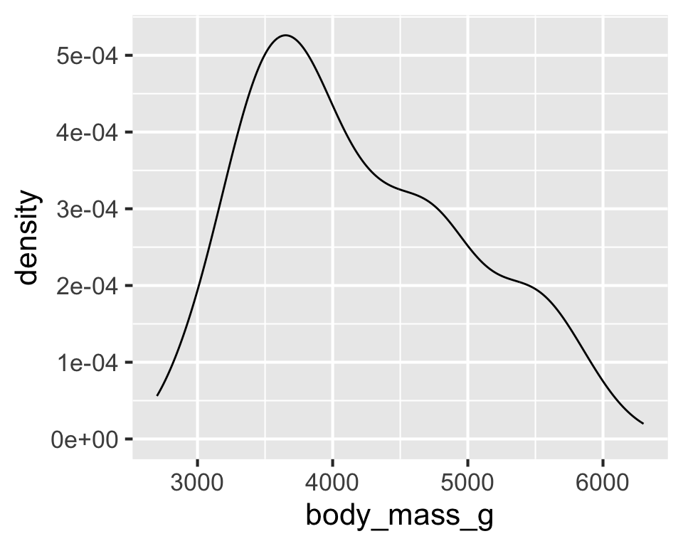
Density plot - Step 2
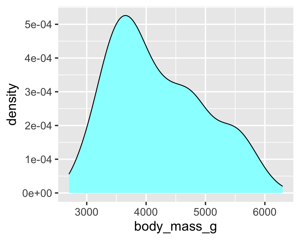
Density plot - Step 3
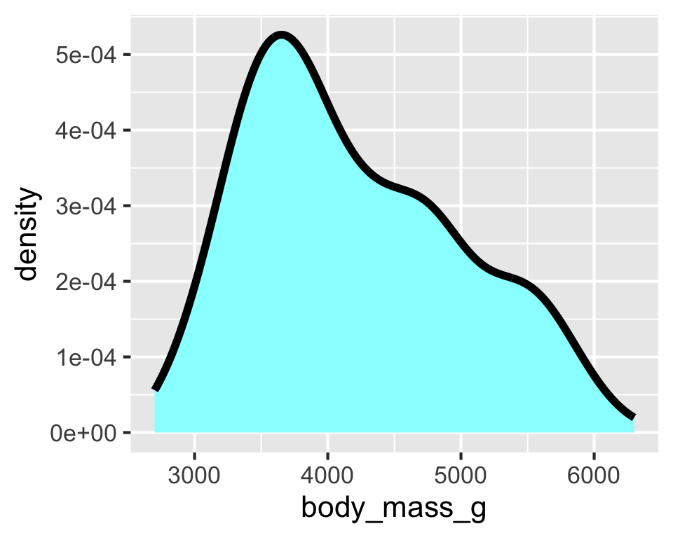
Density plot - Step 4
Density plot - Step 5
Density plot - Step 6
Density plot - Step 7
Weights of penguins
Bivariate analysis
Bivariate analysis
Analyzing the relationship between two variables:
Numerical + numerical: scatterplot
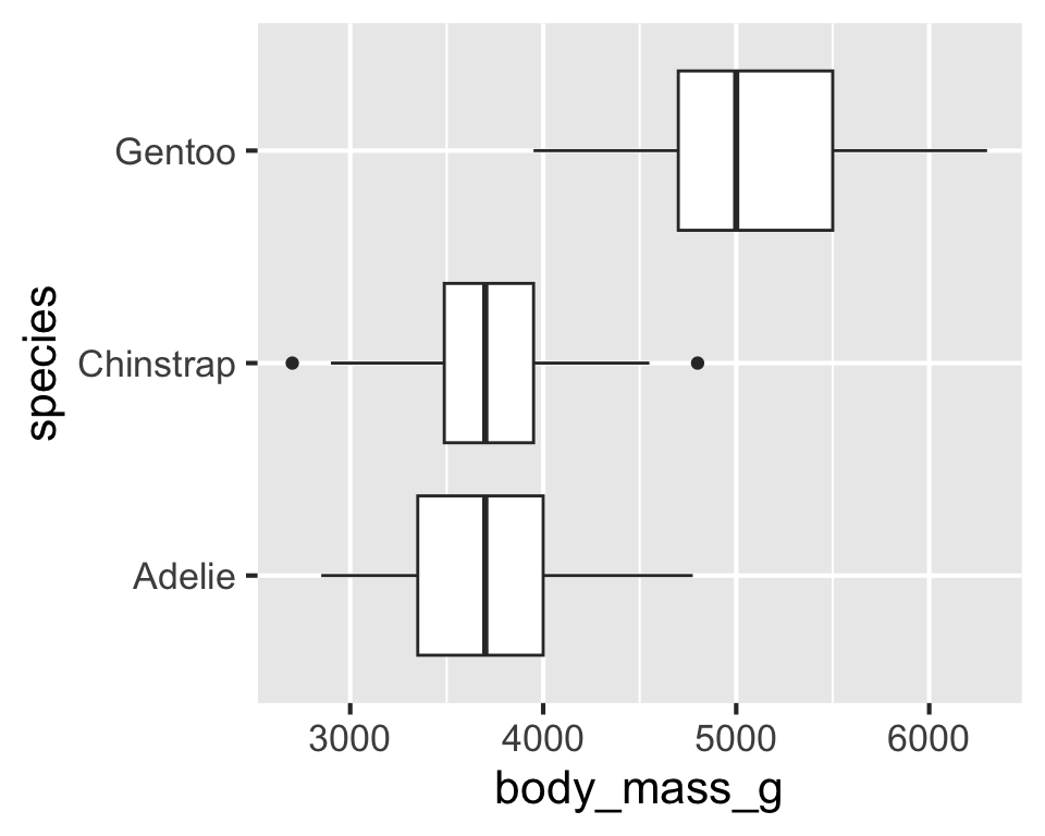
Numerical + categorical: side-by-side box plots, violin plots, etc.
Categorical + categorical: stacked bar plots
Using an aesthetic (e.g., fill, color, shape, etc.) or facets to represent the second variable in any plot
Side-by-side box plots
Density plots
Density plots
Density plots
Density plots

