Grammar of data wrangling

Lecture 5

Dr. Mine Çetinkaya-Rundel

Duke University
STA 199 - Spring 2024

2024-01-30

Warm up

While you wait for class to begin…

Go to your ae repo, click Pull to get today’s application exercise to get ready for later.
Questions from the prepare materials?

Asking good questions

Post content questions on Ed Discussion
If you have a coding question always provide the code, and if relevant, the error
- If this feels impossible, don’t fret it, it’s ok to ask questions without the code. It’s just more efficient with it!
Title your thread in a way that can help others (e.g., “Q7” vs. “error with mutate() function in Lab 1 - Q7”)
Check for previous questions

Coding style + workflow

Avoid long lines of code.
- We should be able to see all of your code in the PDF document you submit.
Label code chunks.
- Do not put spaces in the code-chunk labels.
Render, commit, and push regularly.
- Think about it like clicking to save regularly as you type a report.

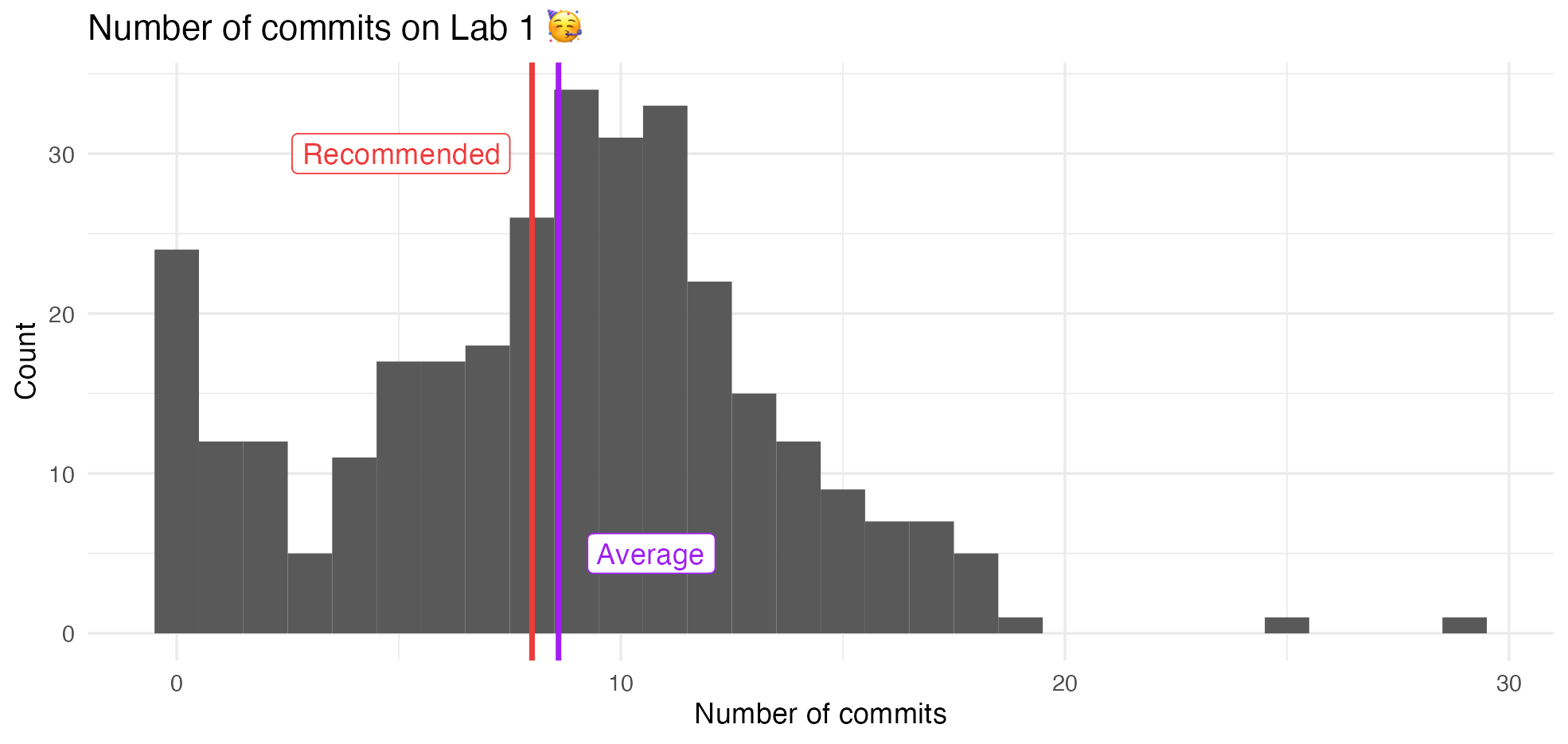
Lab 1

Data frames and `tibble`s

NYC Flights

To demonstrate data wrangling we will use flights, a tibble in the nycflights13 R package.
The data set includes characteristics of all flights departing from New York City (JFK, LGA, EWR) in 2013.

library(tidyverse)
library(nycflights13)

`flights` – dimensions

Number of rows:

nrow(flights)

[1] 336776

Number of columns:

ncol(flights)

[1] 19

glimpse(flights)

Rows: 336,776
Columns: 19
$ year           <int> 2013, 2013, 2013, 2013, 2013, 2013, 2013, 2013, 2013, 2013, 2013,…
$ month          <int> 1, 1, 1, 1, 1, 1, 1, 1, 1, 1, 1, 1, 1, 1, 1, 1, 1, 1, 1, 1, 1, 1,…
$ day            <int> 1, 1, 1, 1, 1, 1, 1, 1, 1, 1, 1, 1, 1, 1, 1, 1, 1, 1, 1, 1, 1, 1,…
$ dep_time       <int> 517, 533, 542, 544, 554, 554, 555, 557, 557, 558, 558, 558, 558, …
$ sched_dep_time <int> 515, 529, 540, 545, 600, 558, 600, 600, 600, 600, 600, 600, 600, …
$ dep_delay      <dbl> 2, 4, 2, -1, -6, -4, -5, -3, -3, -2, -2, -2, -2, -2, -1, 0, -1, 0…
$ arr_time       <int> 830, 850, 923, 1004, 812, 740, 913, 709, 838, 753, 849, 853, 924,…
$ sched_arr_time <int> 819, 830, 850, 1022, 837, 728, 854, 723, 846, 745, 851, 856, 917,…
$ arr_delay      <dbl> 11, 20, 33, -18, -25, 12, 19, -14, -8, 8, -2, -3, 7, -14, 31, -4,…
$ carrier        <chr> "UA", "UA", "AA", "B6", "DL", "UA", "B6", "EV", "B6", "AA", "B6",…
$ flight         <int> 1545, 1714, 1141, 725, 461, 1696, 507, 5708, 79, 301, 49, 71, 194…
$ tailnum        <chr> "N14228", "N24211", "N619AA", "N804JB", "N668DN", "N39463", "N516…
$ origin         <chr> "EWR", "LGA", "JFK", "JFK", "LGA", "EWR", "EWR", "LGA", "JFK", "L…
$ dest           <chr> "IAH", "IAH", "MIA", "BQN", "ATL", "ORD", "FLL", "IAD", "MCO", "O…
$ air_time       <dbl> 227, 227, 160, 183, 116, 150, 158, 53, 140, 138, 149, 158, 345, 3…
$ distance       <dbl> 1400, 1416, 1089, 1576, 762, 719, 1065, 229, 944, 733, 1028, 1005…
$ hour           <dbl> 5, 5, 5, 5, 6, 5, 6, 6, 6, 6, 6, 6, 6, 6, 6, 5, 6, 6, 6, 6, 6, 6,…
$ minute         <dbl> 15, 29, 40, 45, 0, 58, 0, 0, 0, 0, 0, 0, 0, 0, 0, 59, 0, 0, 0, 0,…
$ time_hour      <dttm> 2013-01-01 05:00:00, 2013-01-01 05:00:00, 2013-01-01 05:00:00, 2…

names(flights)

 [1] "year"           "month"          "day"            "dep_time"       "sched_dep_time"
 [6] "dep_delay"      "arr_time"       "sched_arr_time" "arr_delay"      "carrier"       
[11] "flight"         "tailnum"        "origin"         "dest"           "air_time"      
[16] "distance"       "hour"           "minute"         "time_hour"

head(flights)

# A tibble: 6 × 19
   year month   day dep_time sched_dep_time dep_delay arr_time sched_arr_time arr_delay
  <int> <int> <int>    <int>          <int>     <dbl>    <int>          <int>     <dbl>
1  2013     1     1      517            515         2      830            819        11
2  2013     1     1      533            529         4      850            830        20
3  2013     1     1      542            540         2      923            850        33
4  2013     1     1      544            545        -1     1004           1022       -18
5  2013     1     1      554            600        -6      812            837       -25
6  2013     1     1      554            558        -4      740            728        12
# ℹ 10 more variables: carrier <chr>, flight <int>, tailnum <chr>, origin <chr>,
#   dest <chr>, air_time <dbl>, distance <dbl>, hour <dbl>, minute <dbl>,
#   time_hour <dttm>

`tibble` vs. data frame

tibble: an opinionated version of the R data frame
All tibbles are data frames, but not all data frames are tibbles!
Two main differences between a tibble and a data frame:
- Printing
- Stricter subsetting

Printing

tibble
data.frame

Display first 10 rows and all of the columns that fit on the screen will display, along with the type of each column.

flights

# A tibble: 336,776 × 19
    year month   day dep_time sched_dep_time dep_delay arr_time sched_arr_time arr_delay
   <int> <int> <int>    <int>          <int>     <dbl>    <int>          <int>     <dbl>
 1  2013     1     1      517            515         2      830            819        11
 2  2013     1     1      533            529         4      850            830        20
 3  2013     1     1      542            540         2      923            850        33
 4  2013     1     1      544            545        -1     1004           1022       -18
 5  2013     1     1      554            600        -6      812            837       -25
 6  2013     1     1      554            558        -4      740            728        12
 7  2013     1     1      555            600        -5      913            854        19
 8  2013     1     1      557            600        -3      709            723       -14
 9  2013     1     1      557            600        -3      838            846        -8
10  2013     1     1      558            600        -2      753            745         8
# ℹ 336,766 more rows
# ℹ 10 more variables: carrier <chr>, flight <int>, tailnum <chr>, origin <chr>,
#   dest <chr>, air_time <dbl>, distance <dbl>, hour <dbl>, minute <dbl>,
#   time_hour <dttm>

(Attempt to) display all of the data, or die (crash) tryin (if the dataset is too large)!

cars

   speed dist
1      4    2
2      4   10
3      7    4
4      7   22
5      8   16
6      9   10
7     10   18
8     10   26
9     10   34
10    11   17
11    11   28
12    12   14
13    12   20
14    12   24
15    12   28
16    13   26
17    13   34
18    13   34
19    13   46
20    14   26
21    14   36
22    14   60
23    14   80
24    15   20
25    15   26
26    15   54
27    16   32
28    16   40
29    17   32
30    17   40
31    17   50
32    18   42
33    18   56
34    18   76
35    18   84
36    19   36
37    19   46
38    19   68
39    20   32
40    20   48
41    20   52
42    20   56
43    20   64
44    22   66
45    23   54
46    24   70
47    24   92
48    24   93
49    24  120
50    25   85

Stricter subsetting

tibble
data.frame

Warning + NULL if variable not found.

flights$apple

Warning: Unknown or uninitialised column: `apple`.

NULL

Only NULL if variable not found.

cars$apple

NULL

Data wrangling with `dplyr`

dplyr

Primary package in the tidyverse for data wrangling

dplyr.tidyverse.org

Cheat sheet

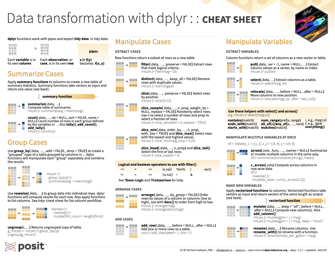
Row operations

slice(): chooses rows based on location
filter():chooses rows based on column values
arrange(): changes the order of the rows
sample_n(): take a random subset of the rows

`slice()`

Display the first five rows of flights:

1flights |>
2  slice(1:5)

1: Take the flights data frame, and then,
2: Slice its first five rows

# A tibble: 5 × 19
   year month   day dep_time sched_dep_time dep_delay arr_time sched_arr_time arr_delay
  <int> <int> <int>    <int>          <int>     <dbl>    <int>          <int>     <dbl>
1  2013     1     1      517            515         2      830            819        11
2  2013     1     1      533            529         4      850            830        20
3  2013     1     1      542            540         2      923            850        33
4  2013     1     1      544            545        -1     1004           1022       -18
5  2013     1     1      554            600        -6      812            837       -25
# ℹ 10 more variables: carrier <chr>, flight <int>, tailnum <chr>, origin <chr>,
#   dest <chr>, air_time <dbl>, distance <dbl>, hour <dbl>, minute <dbl>,
#   time_hour <dttm>

`filter()`

Filter for flights to RDU in flights:

1flights |>
2  filter(dest == "RDU")

1: Take the flights data frame, and then,
2: Filter for rows where dest is equal to RDU

# A tibble: 8,163 × 19
    year month   day dep_time sched_dep_time dep_delay arr_time sched_arr_time arr_delay
   <int> <int> <int>    <int>          <int>     <dbl>    <int>          <int>     <dbl>
 1  2013     1     1      800            810       -10      949            955        -6
 2  2013     1     1      832            840        -8     1006           1030       -24
 3  2013     1     1      851            851         0     1032           1036        -4
 4  2013     1     1      917            920        -3     1052           1108       -16
 5  2013     1     1     1024           1030        -6     1204           1215       -11
 6  2013     1     1     1127           1129        -2     1303           1309        -6
 7  2013     1     1     1157           1205        -8     1342           1345        -3
 8  2013     1     1     1240           1235         5     1415           1415         0
 9  2013     1     1     1317           1325        -8     1454           1505       -11
10  2013     1     1     1449           1450        -1     1651           1640        11
# ℹ 8,153 more rows
# ℹ 10 more variables: carrier <chr>, flight <int>, tailnum <chr>, origin <chr>,
#   dest <chr>, air_time <dbl>, distance <dbl>, hour <dbl>, minute <dbl>,
#   time_hour <dttm>

The pipe

The pipe, |>, is an operator (a tool) for passing information from one process to another.
Use |> mainly in data pipelines to pass the output of the previous line of code as the first input of the next line of code.
When reading code “in English”, say “and then” whenever you see a pipe.

Delayed flights to RDU

Which airline is the most delayed, on average, arriving in RDU from a New York City airport?

Goal:

# A tibble: 5 × 2
  carrier mean_arr_delay
  <chr>            <dbl>
1 UA               56   
2 B6               13.3 
3 EV               12.2 
4 9E                9.67
5 MQ                8.82

The pipe, in action

1flights

1: Take the flights data frame

# A tibble: 336,776 × 19
    year month   day dep_time sched_dep_time dep_delay arr_time sched_arr_time arr_delay
   <int> <int> <int>    <int>          <int>     <dbl>    <int>          <int>     <dbl>
 1  2013     1     1      517            515         2      830            819        11
 2  2013     1     1      533            529         4      850            830        20
 3  2013     1     1      542            540         2      923            850        33
 4  2013     1     1      544            545        -1     1004           1022       -18
 5  2013     1     1      554            600        -6      812            837       -25
 6  2013     1     1      554            558        -4      740            728        12
 7  2013     1     1      555            600        -5      913            854        19
 8  2013     1     1      557            600        -3      709            723       -14
 9  2013     1     1      557            600        -3      838            846        -8
10  2013     1     1      558            600        -2      753            745         8
# ℹ 336,766 more rows
# ℹ 10 more variables: carrier <chr>, flight <int>, tailnum <chr>, origin <chr>,
#   dest <chr>, air_time <dbl>, distance <dbl>, hour <dbl>, minute <dbl>,
#   time_hour <dttm>

The pipe, in action

1flights |>
2  filter(dest == "RDU")

1: Take the flights data frame,
2: and then filter for flights going to RDU

# A tibble: 8,163 × 19
    year month   day dep_time sched_dep_time dep_delay arr_time sched_arr_time arr_delay
   <int> <int> <int>    <int>          <int>     <dbl>    <int>          <int>     <dbl>
 1  2013     1     1      800            810       -10      949            955        -6
 2  2013     1     1      832            840        -8     1006           1030       -24
 3  2013     1     1      851            851         0     1032           1036        -4
 4  2013     1     1      917            920        -3     1052           1108       -16
 5  2013     1     1     1024           1030        -6     1204           1215       -11
 6  2013     1     1     1127           1129        -2     1303           1309        -6
 7  2013     1     1     1157           1205        -8     1342           1345        -3
 8  2013     1     1     1240           1235         5     1415           1415         0
 9  2013     1     1     1317           1325        -8     1454           1505       -11
10  2013     1     1     1449           1450        -1     1651           1640        11
# ℹ 8,153 more rows
# ℹ 10 more variables: carrier <chr>, flight <int>, tailnum <chr>, origin <chr>,
#   dest <chr>, air_time <dbl>, distance <dbl>, hour <dbl>, minute <dbl>,
#   time_hour <dttm>

The pipe, in action

1flights |>
2  filter(dest == "RDU") |>
3  group_by(carrier)

1: Take the flights data frame,
2: and then filter for flights going to RDU,
3: and then group by carrier

# A tibble: 8,163 × 19
# Groups:   carrier [5]
    year month   day dep_time sched_dep_time dep_delay arr_time sched_arr_time arr_delay
   <int> <int> <int>    <int>          <int>     <dbl>    <int>          <int>     <dbl>
 1  2013     1     1      800            810       -10      949            955        -6
 2  2013     1     1      832            840        -8     1006           1030       -24
 3  2013     1     1      851            851         0     1032           1036        -4
 4  2013     1     1      917            920        -3     1052           1108       -16
 5  2013     1     1     1024           1030        -6     1204           1215       -11
 6  2013     1     1     1127           1129        -2     1303           1309        -6
 7  2013     1     1     1157           1205        -8     1342           1345        -3
 8  2013     1     1     1240           1235         5     1415           1415         0
 9  2013     1     1     1317           1325        -8     1454           1505       -11
10  2013     1     1     1449           1450        -1     1651           1640        11
# ℹ 8,153 more rows
# ℹ 10 more variables: carrier <chr>, flight <int>, tailnum <chr>, origin <chr>,
#   dest <chr>, air_time <dbl>, distance <dbl>, hour <dbl>, minute <dbl>,
#   time_hour <dttm>

The pipe, in action

1flights |>
2  filter(dest == "RDU") |>
3  group_by(carrier) |>
4  summarize(mean_arr_delay = mean(arr_delay, na.rm = TRUE))

1: Take the flights data frame,
2: and then filter for flights going to RDU,
3: and then group by carrier,
4: and then calculate the mean arrival delay for each carrier

# A tibble: 5 × 2
  carrier mean_arr_delay
  <chr>            <dbl>
1 9E                9.67
2 B6               13.3 
3 EV               12.2 
4 MQ                8.82
5 UA               56

The pipe, in action

1flights |>
2  filter(dest == "RDU") |>
3  group_by(carrier) |>
4  summarize(mean_arr_delay = mean(arr_delay, na.rm = TRUE)) |>
5  arrange(desc(mean_arr_delay))

1: Take the flights data frame,
2: and then filter for flights going to RDU,
3: and then group by carrier,
4: and then calculate the mean arrival delay for each carrier,
5: and then arrange in descending order of mean arrival delay.

# A tibble: 5 × 2
  carrier mean_arr_delay
  <chr>            <dbl>
1 UA               56   
2 B6               13.3 
3 EV               12.2 
4 9E                9.67
5 MQ                8.82

Column operations

select(): changes whether or not a column is included.
rename(): changes the name of columns.
mutate(): changes the values of columns and creates new columns.

Groups of rows

summarize(): collapses a group into a single row.
count(): count unique values of one or more variables.
group_by(): perform calculations separately for each value of a variable

Application exercise

`ae-04-flights-wrangling`

Go to the project navigator in RStudio (top right corner of your RStudio window) and open the project called ae.
If there are any uncommitted files, commit them, and then click Pull.
Open the file called ae-04-flights-wrangling.qmd and render it.

Recap: pipe

The pipe operator passes what comes before it into the function that comes after it as the first argument in that function.

sum(1, 2)

[1] 3

1 |> 
  sum(2)

[1] 3

Always use a line break after the pipe, and indent the next line of code.
- Just like always use a line break between layers of ggplots, after +, and indent the next line.

Recap: logical operators

operator	definition
`<`	is less than?
`<=`	is less than or equal to?
`>`	is greater than?
`>=`	is greater than or equal to?
`==`	is exactly equal to?
`!=`	is not equal to?

Recap: logical operators

operator	definition
`x & y`	is x AND y?
`x \\| y`	is x OR y?
`is.na(x)`	is x NA?
`!is.na(x)`	is x not NA?
`x %in% y`	is x in y?
`!(x %in% y)`	is x not in y?
`!x`	is not x? (only makes sense if `x` is `TRUE` or `FALSE`)

Grammar of data wrangling

Warm up

While you wait for class to begin…

Asking good questions

Coding style + workflow

Lab 1

Data frames and tibbles

NYC Flights

flights – dimensions

flights – first look

tibble vs. data frame

Printing

Stricter subsetting

Data wrangling with dplyr

dplyr

Row operations

slice()

filter()

The pipe

Delayed flights to RDU

The pipe, in action

The pipe, in action

The pipe, in action

The pipe, in action

The pipe, in action

Column operations

Groups of rows

Application exercise

ae-04-flights-wrangling

Recap: pipe

Recap: logical operators

Recap: logical operators

Data frames and `tibble`s

`flights` – dimensions

`flights` – first look

`tibble` vs. data frame

Data wrangling with `dplyr`

`slice()`

`filter()`

`ae-04-flights-wrangling`