Tidying data

Lecture 6

Dr. Mine Çetinkaya-Rundel

Duke University
STA 199 - Spring 2024

2024-02-01

Warm up

While you wait for class to begin…

Go to your ae repo, click Pull to get today’s application exercise to get ready for later.
Questions from the prepare materials?

Announcements

Lab 2 due Monday, 8 am

From last time: Application exercise

`ae-04-flights-wrangling`

Go to the project navigator in RStudio (top right corner of your RStudio window) and open the project called ae.
Open the file called ae-04-flights-wrangling.qmd and render it.

Recap: pipe

The pipe operator passes what comes before it into the function that comes after it as the first argument in that function.

sum(1, 2)

[1] 3

1 |> 
  sum(2)

[1] 3

Always use a line break after the pipe, and indent the next line of code.
- Just like always use a line break between layers of ggplots, after +, and indent the next line.

Recap: logical operators

operator	definition
`<`	is less than?
`<=`	is less than or equal to?
`>`	is greater than?
`>=`	is greater than or equal to?
`==`	is exactly equal to?
`!=`	is not equal to?

Recap: logical operators

operator	definition
`x & y`	is x AND y?
`x \\| y`	is x OR y?
`is.na(x)`	is x NA?
`!is.na(x)`	is x not NA?
`x %in% y`	is x in y?
`!(x %in% y)`	is x not in y?
`!x`	is not x? (only makes sense if `x` is `TRUE` or `FALSE`)

Recap: assignment

Let’s make a tiny data frame to use as an example:

library(tidyverse)
df <- tibble(x = c(1, 2, 3, 4, 5), y = c("a", "a", "b", "c", "c"))
df

# A tibble: 5 × 2
      x y    
  <dbl> <chr>
1     1 a    
2     2 a    
3     3 b    
4     4 c    
5     5 c

Recap: assignment

Do something and show me

df |>
  mutate(x = x * 2)

# A tibble: 5 × 2
      x y    
  <dbl> <chr>
1     2 a    
2     4 a    
3     6 b    
4     8 c    
5    10 c

df

# A tibble: 5 × 2
      x y    
  <dbl> <chr>
1     1 a    
2     2 a    
3     3 b    
4     4 c    
5     5 c

Do something and save result

df <- df |>
  mutate(x = x * 2)
df

# A tibble: 5 × 2
      x y    
  <dbl> <chr>
1     2 a    
2     4 a    
3     6 b    
4     8 c    
5    10 c

Recap: assignment

Do something, save result, overwriting original

df <- tibble(
  x = c(1, 2, 3, 4, 5), 
  y = c("a", "a", "b", "c", "c")
)
df <- df |>
  mutate(x = x * 2)
df

# A tibble: 5 × 2
      x y    
  <dbl> <chr>
1     2 a    
2     4 a    
3     6 b    
4     8 c    
5    10 c

Do something, save result, not overwriting original

df <- tibble(
  x = c(1, 2, 3, 4, 5), 
  y = c("a", "a", "b", "c", "c")
)
df_new <- df |>
  mutate(x = x * 2)
df_new

# A tibble: 5 × 2
      x y    
  <dbl> <chr>
1     2 a    
2     4 a    
3     6 b    
4     8 c    
5    10 c

Recap: assignment

Do something, save result, overwriting original when you shouldn’t

df <- tibble(
  x = c(1, 2, 3, 4, 5), 
  y = c("a", "a", "b", "c", "c")
)
df <- df |>
  group_by(y) |>
  summarize(mean_x = mean(x))
df

# A tibble: 3 × 2
  y     mean_x
  <chr>  <dbl>
1 a        1.5
2 b        3  
3 c        4.5

Do something, save result, not overwriting original when you shouldn’t

df <- tibble(
  x = c(1, 2, 3, 4, 5), 
  y = c("a", "a", "b", "c", "c")
)
df_summary <- df |>
  group_by(y) |>
  summarize(mean_x = mean(x))
df_summary

# A tibble: 3 × 2
  y     mean_x
  <chr>  <dbl>
1 a        1.5
2 b        3  
3 c        4.5

Recap: assignment

Do something, save result, overwriting original
data frame

df <- tibble(
  x = c(1, 2, 3, 4, 5), 
  y = c("a", "a", "b", "c", "c")
)
df <- df |>
  mutate(z = x + 2)
df

# A tibble: 5 × 3
      x y         z
  <dbl> <chr> <dbl>
1     1 a         3
2     2 a         4
3     3 b         5
4     4 c         6
5     5 c         7

Do something, save result, overwriting original
column

df <- tibble(
  x = c(1, 2, 3, 4, 5), 
  y = c("a", "a", "b", "c", "c")
)
df <- df |>
  mutate(x = x + 2)
df

# A tibble: 5 × 2
      x y    
  <dbl> <chr>
1     3 a    
2     4 a    
3     5 b    
4     6 c    
5     7 c

Data tidying

Tidy data

“Tidy datasets are easy to manipulate, model and visualise, and have a specific structure: each variable is a column, each observation is a row, and each type of observational unit is a table.”

Tidy Data, https://vita.had.co.nz/papers/tidy-data.pdf

Note: “easy to manipulate” = “straightforward to manipulate”

Goal

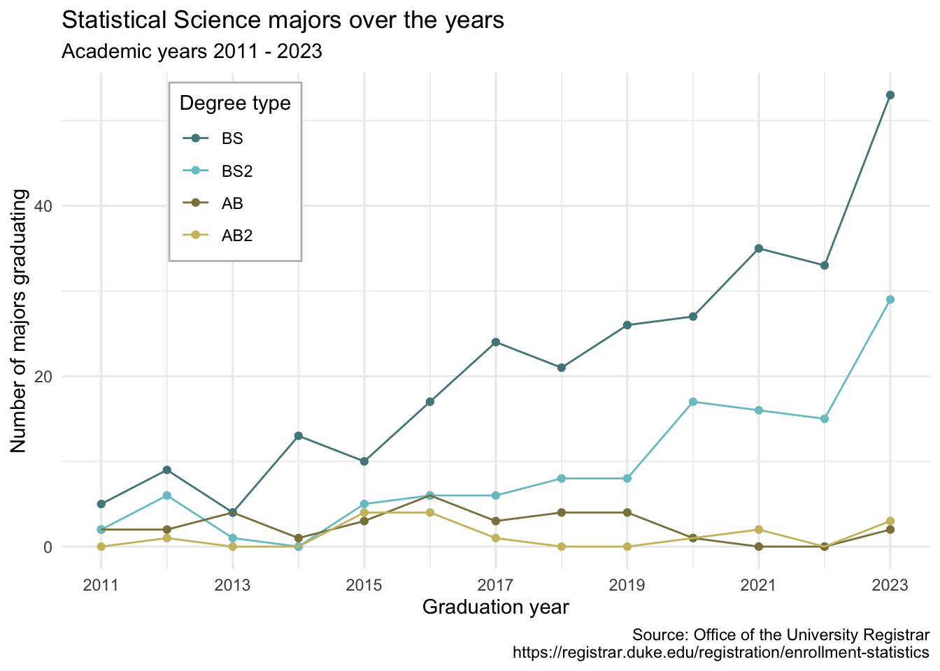
Visualize StatSci majors over the years!

Data

statsci <- read_csv("https://sta199-s24.github.io/data/statsci.csv")
statsci

# A tibble: 4 × 14
  degree      `2011` `2012` `2013` `2014` `2015` `2016` `2017` `2018` `2019` `2020` `2021`
  <chr>        <dbl>  <dbl>  <dbl>  <dbl>  <dbl>  <dbl>  <dbl>  <dbl>  <dbl>  <dbl>  <dbl>
1 Statistica…     NA      1     NA     NA      4      4      1     NA     NA      1      2
2 Statistica…      2      2      4      1      3      6      3      4      4      1     NA
3 Statistica…      2      6      1     NA      5      6      6      8      8     17     16
4 Statistica…      5      9      4     13     10     17     24     21     26     27     35
# ℹ 2 more variables: `2022` <dbl>, `2023` <dbl>

The first column (variable) is the degree, and there are 4 possible degrees: BS (Bachelor of Science), BS2 (Bachelor of Science, 2nd major), AB (Bachelor of Arts), AB2 (Bachelor of Arts, 2nd major).
The remaining columns show the number of students graduating with that major in a given academic year from 2011 to 2023.

Let’s plan!

Take a look at the plot we aim to make and sketch the data frame we need to make the plot. Determine what each row and each column of the data frame should be. Hint: We need data to be in columns to map to aesthetic elements of the plot.

Application exercise

`ae-05-majors-tidying`

Go to the project navigator in RStudio (top right corner of your RStudio window) and open the project called ae.
If there are any uncommitted files, commit them, and then click Pull.
Open the file called ae-05-majors-tidying.qmd and render it.

Recap: pivoting

Data sets can’t be labeled as wide or long but they can be made wider or longer for a certain analysis that requires a certain format
When pivoting longer, variable names that turn into values are characters by default. If you need them to be in another format, you need to explicitly make that transformation, which you can do so within the pivot_longer() function.
You can tweak a plot forever, but at some point the tweaks are likely not very productive. However, you should always be critical of defaults (however pretty they might be) and see if you can improve the plot to better portray your data / results / what you want to communicate.