Joining data

Lecture 7

Dr. Mine Çetinkaya-Rundel

Duke University
STA 199 - Spring 2024

2024-02-06

Warm up

While you wait for class to begin…

Go to your ae repo, click Pull to get today’s application exercise to get ready for later.
Questions from the prepare materials?

Announcements

Exam 1 in class next week on Thursday – cheat sheet (1 page, both sides, hand-written or typed, must be prepared by you)
Exam 1 take home starts after class on Thursday, due at 8 am on Monday (open resources, internet, etc., closed to other humans)
Next week in lab: Exam 1 review – come with questions!
No new lab assigned next week during exam

Study tips for the exam

Go over lecture materials and application exercises
Review labs and feedback you’ve received so far
Do the exercises at the end of readings from both books
Do the exam review over (to be posted on Friday)
Go to lab on Monday with questions

Questions from last time

Is there a limit to a tibble size?

No, a tibble (i.e., a data frame) can be any number of rows or columns. However when you print it, it will only print the first 10 rows and the columns that fit across the screen, document, etc.

If you want to see more rows and columns, you can

open it in the data viewer with view(df)
explicitly print more rows with, e.g., df |> print(n = 25)
explicitly select() or relocate() columns

library(tidyverse)
midwest

# A tibble: 437 × 28
     PID county   state  area poptotal popdensity popwhite popblack popamerindian popasian
   <int> <chr>    <chr> <dbl>    <int>      <dbl>    <int>    <int>         <int>    <int>
 1   561 ADAMS    IL    0.052    66090      1271.    63917     1702            98      249
 2   562 ALEXAND… IL    0.014    10626       759      7054     3496            19       48
 3   563 BOND     IL    0.022    14991       681.    14477      429            35       16
 4   564 BOONE    IL    0.017    30806      1812.    29344      127            46      150
 5   565 BROWN    IL    0.018     5836       324.     5264      547            14        5
 6   566 BUREAU   IL    0.05     35688       714.    35157       50            65      195
 7   567 CALHOUN  IL    0.017     5322       313.     5298        1             8       15
 8   568 CARROLL  IL    0.027    16805       622.    16519      111            30       61
 9   569 CASS     IL    0.024    13437       560.    13384       16             8       23
10   570 CHAMPAI… IL    0.058   173025      2983.   146506    16559           331     8033
# ℹ 427 more rows
# ℹ 18 more variables: popother <int>, percwhite <dbl>, percblack <dbl>,
#   percamerindan <dbl>, percasian <dbl>, percother <dbl>, popadults <int>,
#   perchsd <dbl>, percollege <dbl>, percprof <dbl>, poppovertyknown <int>,
#   percpovertyknown <dbl>, percbelowpoverty <dbl>, percchildbelowpovert <dbl>,
#   percadultpoverty <dbl>, percelderlypoverty <dbl>, inmetro <int>, category <chr>

midwest |>
  print(n = 13)

# A tibble: 437 × 28
     PID county   state  area poptotal popdensity popwhite popblack popamerindian popasian
   <int> <chr>    <chr> <dbl>    <int>      <dbl>    <int>    <int>         <int>    <int>
 1   561 ADAMS    IL    0.052    66090      1271.    63917     1702            98      249
 2   562 ALEXAND… IL    0.014    10626       759      7054     3496            19       48
 3   563 BOND     IL    0.022    14991       681.    14477      429            35       16
 4   564 BOONE    IL    0.017    30806      1812.    29344      127            46      150
 5   565 BROWN    IL    0.018     5836       324.     5264      547            14        5
 6   566 BUREAU   IL    0.05     35688       714.    35157       50            65      195
 7   567 CALHOUN  IL    0.017     5322       313.     5298        1             8       15
 8   568 CARROLL  IL    0.027    16805       622.    16519      111            30       61
 9   569 CASS     IL    0.024    13437       560.    13384       16             8       23
10   570 CHAMPAI… IL    0.058   173025      2983.   146506    16559           331     8033
11   571 CHRISTI… IL    0.042    34418       819.    34176       82            51       89
12   572 CLARK    IL    0.03     15921       531.    15842       10            26       36
13   573 CLAY     IL    0.028    14460       516.    14403        4            17       29
# ℹ 424 more rows
# ℹ 18 more variables: popother <int>, percwhite <dbl>, percblack <dbl>,
#   percamerindan <dbl>, percasian <dbl>, percother <dbl>, popadults <int>,
#   perchsd <dbl>, percollege <dbl>, percprof <dbl>, poppovertyknown <int>,
#   percpovertyknown <dbl>, percbelowpoverty <dbl>, percchildbelowpovert <dbl>,
#   percadultpoverty <dbl>, percelderlypoverty <dbl>, inmetro <int>, category <chr>

midwest |>
  select(county, state, percbelowpoverty, percollege)

# A tibble: 437 × 4
   county    state percbelowpoverty percollege
   <chr>     <chr>            <dbl>      <dbl>
 1 ADAMS     IL               13.2        19.6
 2 ALEXANDER IL               32.2        11.2
 3 BOND      IL               12.1        17.0
 4 BOONE     IL                7.21       17.3
 5 BROWN     IL               13.5        14.5
 6 BUREAU    IL               10.4        18.9
 7 CALHOUN   IL               15.1        11.9
 8 CARROLL   IL               11.7        16.2
 9 CASS      IL               13.9        14.1
10 CHAMPAIGN IL               15.6        41.3
# ℹ 427 more rows

midwest |>
  relocate(county, state, percbelowpoverty, percollege)

# A tibble: 437 × 28
   county    state percbelowpoverty percollege   PID  area poptotal popdensity popwhite
   <chr>     <chr>            <dbl>      <dbl> <int> <dbl>    <int>      <dbl>    <int>
 1 ADAMS     IL               13.2        19.6   561 0.052    66090      1271.    63917
 2 ALEXANDER IL               32.2        11.2   562 0.014    10626       759      7054
 3 BOND      IL               12.1        17.0   563 0.022    14991       681.    14477
 4 BOONE     IL                7.21       17.3   564 0.017    30806      1812.    29344
 5 BROWN     IL               13.5        14.5   565 0.018     5836       324.     5264
 6 BUREAU    IL               10.4        18.9   566 0.05     35688       714.    35157
 7 CALHOUN   IL               15.1        11.9   567 0.017     5322       313.     5298
 8 CARROLL   IL               11.7        16.2   568 0.027    16805       622.    16519
 9 CASS      IL               13.9        14.1   569 0.024    13437       560.    13384
10 CHAMPAIGN IL               15.6        41.3   570 0.058   173025      2983.   146506
# ℹ 427 more rows
# ℹ 19 more variables: popblack <int>, popamerindian <int>, popasian <int>,
#   popother <int>, percwhite <dbl>, percblack <dbl>, percamerindan <dbl>,
#   percasian <dbl>, percother <dbl>, popadults <int>, perchsd <dbl>, percprof <dbl>,
#   poppovertyknown <int>, percpovertyknown <dbl>, percchildbelowpovert <dbl>,
#   percadultpoverty <dbl>, percelderlypoverty <dbl>, inmetro <int>, category <chr>

From last time: pivoting

Data sets can’t be labeled as wide or long but they can be made wider or longer for a certain analysis that requires a certain format
When pivoting longer, variable names that turn into values are characters by default. If you need them to be in another format, you need to explicitly make that transformation, which you can do so within the pivot_longer() function.
You can tweak a plot forever, but at some point the tweaks are likely not very productive. However, you should always be critical of defaults (however pretty they might be) and see if you can improve the plot to better portray your data / results / what you want to communicate.

Joining datasets

Why join?

Suppose we want to answer questions like:

Is there a relationship between
- number of QS courses taken
- having scored a 4 or 5 on the AP stats exam
- motivation for taking course
- …
and performance in this course?”

Each of these would require joining class performance data with an outside data source so we can have all relevant information (columns) in a single data frame.

Setup

For the next few slides…

x <- tibble(
  id = c(1, 2, 3),
  value_x = c("x1", "x2", "x3")
  )

x

# A tibble: 3 × 2
     id value_x
  <dbl> <chr>  
1     1 x1     
2     2 x2     
3     3 x3

y <- tibble(
  id = c(1, 2, 4),
  value_y = c("y1", "y2", "y4")
  )

y

# A tibble: 3 × 2
     id value_y
  <dbl> <chr>  
1     1 y1     
2     2 y2     
3     4 y4

`left_join()`

left_join(x, y)

# A tibble: 3 × 3
     id value_x value_y
  <dbl> <chr>   <chr>  
1     1 x1      y1     
2     2 x2      y2     
3     3 x3      <NA>

`right_join()`

right_join(x, y)

# A tibble: 3 × 3
     id value_x value_y
  <dbl> <chr>   <chr>  
1     1 x1      y1     
2     2 x2      y2     
3     4 <NA>    y4

`full_join()`

full_join(x, y)

# A tibble: 4 × 3
     id value_x value_y
  <dbl> <chr>   <chr>  
1     1 x1      y1     
2     2 x2      y2     
3     3 x3      <NA>   
4     4 <NA>    y4

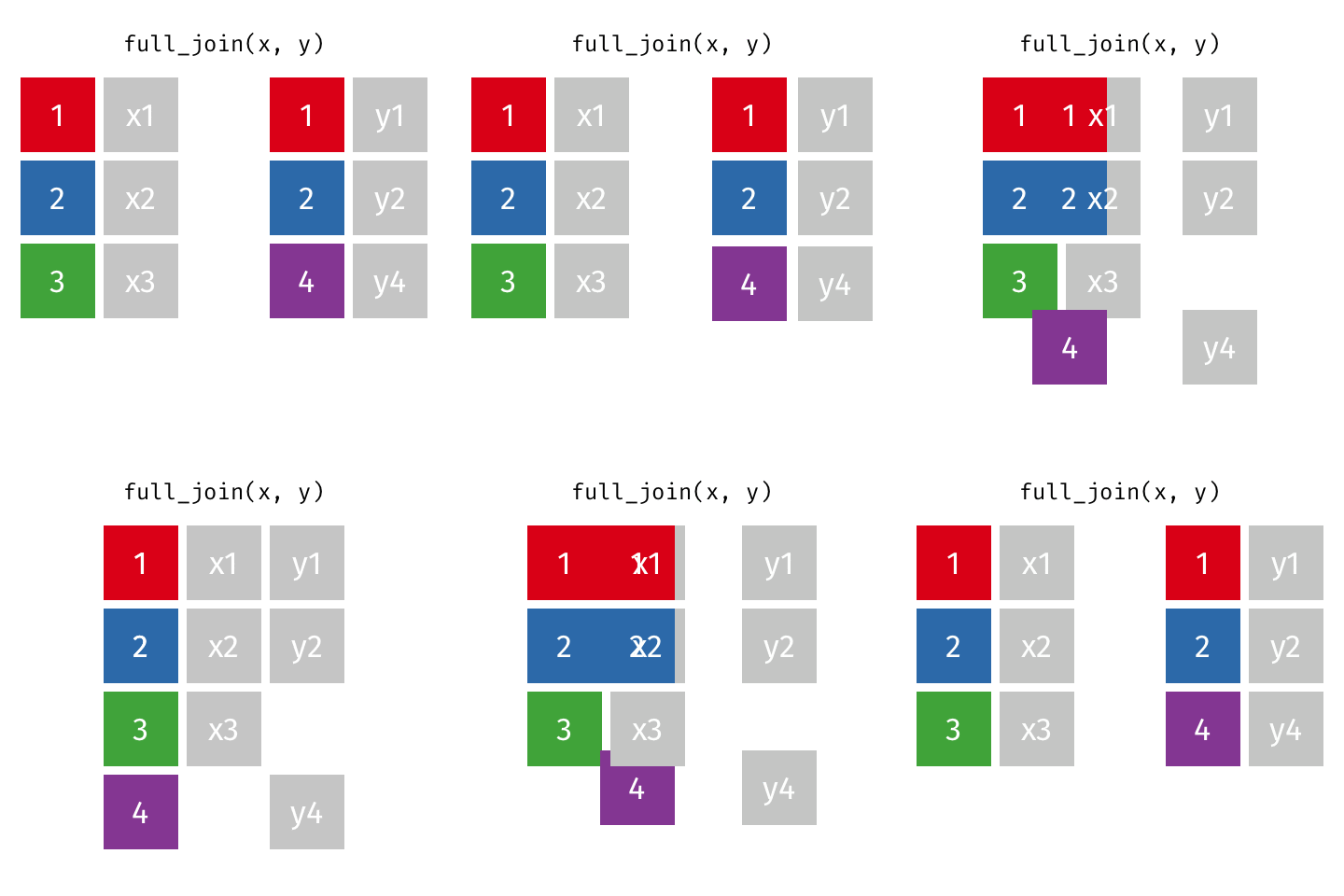
`inner_join()`

inner_join(x, y)

# A tibble: 2 × 3
     id value_x value_y
  <dbl> <chr>   <chr>  
1     1 x1      y1     
2     2 x2      y2

`semi_join()`

semi_join(x, y)

# A tibble: 2 × 2
     id value_x
  <dbl> <chr>  
1     1 x1     
2     2 x2

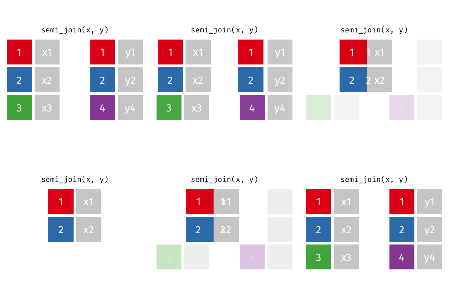
`anti_join()`

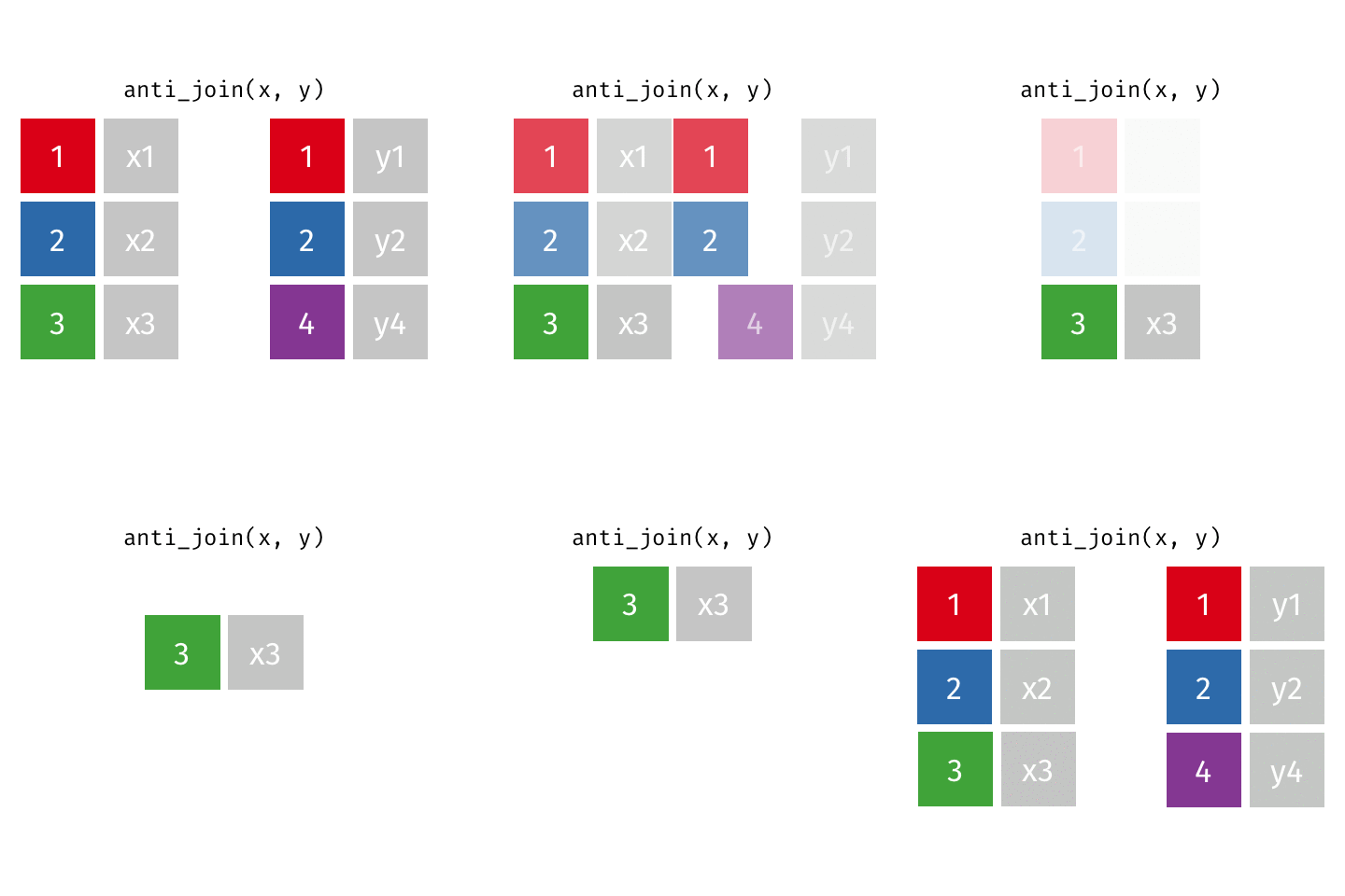
anti_join(x, y)

# A tibble: 1 × 2
     id value_x
  <dbl> <chr>  
1     3 x3

Example: Passenger capacity

`nycflights13` & airport capacity

You’ve previously seen the flights data available in the nycflights13 package which details all flights from one of the 3 major NYC airports in 2013.

Today we would like to answer a specific question:

What was the passenger capacity (i.e., maximum number of passengers) that could have flown out of the three airports in 2013?

To answer this we will need to know how many passenger seats each plane had available - each flight record has a tailnum which is a unique identifier for the plane, this can be linked to the planes data set which has the number of available seats for each plane.

Attempt 1

library(nycflights13)

left_join(flights, planes) |>
  group_by(origin) |>
  summarize(capacity = sum(seats))

# A tibble: 3 × 2
  origin capacity
  <chr>     <int>
1 EWR          NA
2 JFK          NA
3 LGA          NA

Attempt 2

left_join(flights, planes) |>
  group_by(origin) |>
  summarize(capacity = sum(seats, na.rm = TRUE))

# A tibble: 3 × 2
  origin capacity
  <chr>     <int>
1 EWR      345268
2 JFK      179412
3 LGA       89686

Attempt 3

left_join(
  flights, planes,
  by = c("tailnum" = "tailnum")
) |>
  group_by(origin) |>
  summarize(capacity = sum(seats, na.rm = TRUE))

# A tibble: 3 × 2
  origin capacity
  <chr>     <int>
1 EWR    14454251
2 JFK    13874081
3 LGA    10522985

Application exercise

Goal

Make a bar plot of total populations of continents, where the input data are:

Countries and populations
Countries and continents

`ae-06-population-joining`

Go to the project navigator in RStudio (top right corner of your RStudio window) and open the project called ae.
If there are any uncommitted files, commit them, and then click Pull.
Open the file called ae-06-population-joining.qmd and render it.