Linear regression with a single predictor
Lecture 15
Duke University
STA 199 - Spring 2024
2024-03-07
Warm up
Announcements
- We did not finish AE 10 last time, answers are posted for review. Today’s AE 11 will review much of the material we didn’t get to in AE 10.
- The midsemester course feedback survey is open until Sunday midnight. It’s on Canvas > Quizzes, anonymous and optional but participation much appreciated!
Questions from last time
Can you iterate using a function with multiple variables?
Yes, a function can have multiple inputs (just like, for example, the *_join() functions we’ve used take at least two inputs – the two data frames to be joined). We won’t cover writing functions in detail in this class but R4DS - Chp 25 is a good resource for getting started, and STA 323 goes into this topic deeper.
Can you get special permission to scrape (if so, how common is this?)
Probably not? They would just give you the data! Or access to an API where you can fetch the data from.
Questions from last time
Do we have to use OpenIntro for data modelling?
Yes, I recommend the readings from the OpenIntro book for modeling, where relevant they’re linked from the prepare materials.
Goals
- Modeling with a single predictor
- Model parameters, estimates, and error terms
- Interpreting slopes and intercepts
Setup
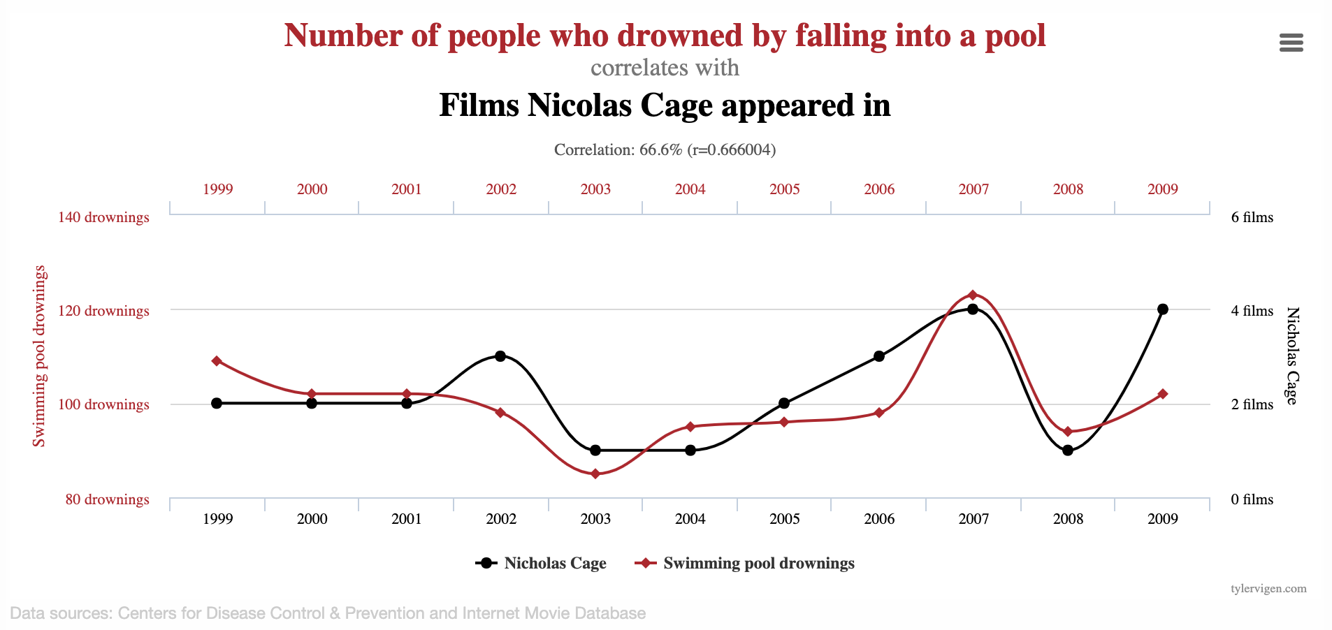
Correlation vs. causation
Spurious correlations

Spurious correlations
Linear regression with a single predictor
Data prep
- Rename Rotten Tomatoes columns as
criticsandaudience - Rename the dataset as
movie_scores
Data overview
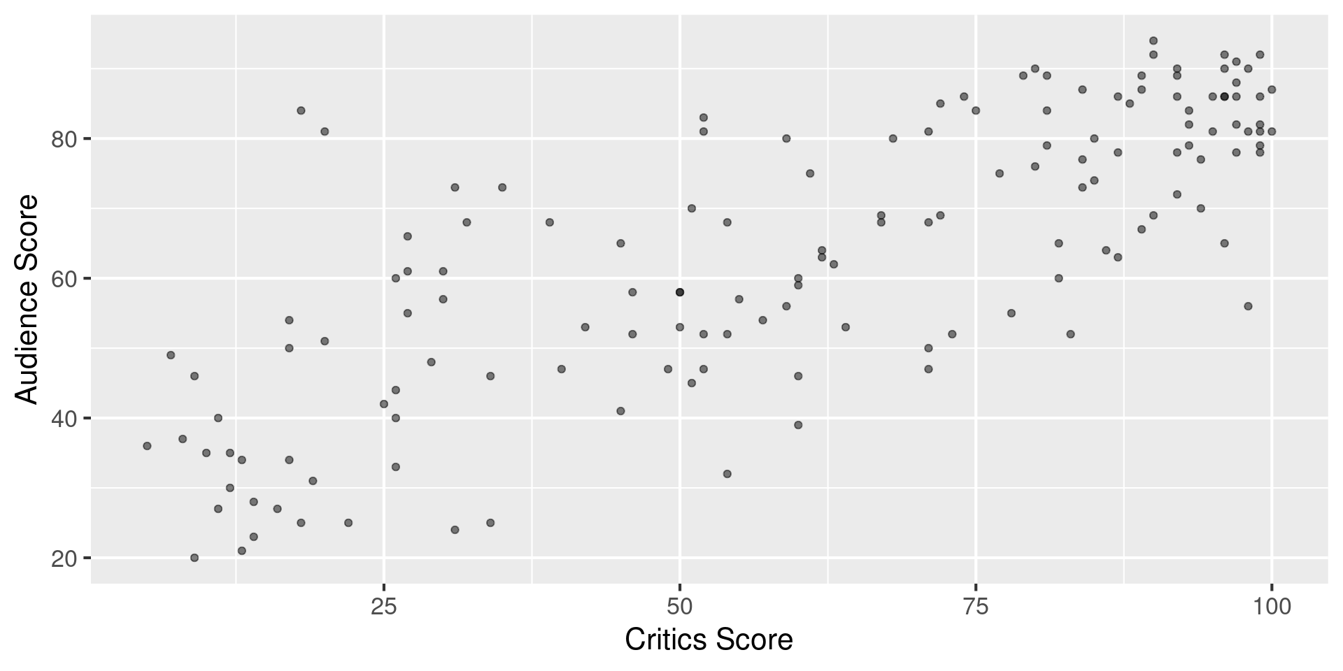
Data visualization
Regression model
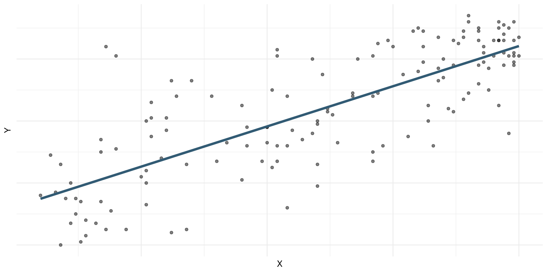
A regression model is a function that describes the relationship between the outcome, \(Y\), and the predictor, \(X\).
\[\begin{aligned} Y &= \color{black}{\textbf{Model}} + \text{Error} \\[8pt] &= \color{black}{\mathbf{f(X)}} + \epsilon \\[8pt] &= \color{black}{\boldsymbol{\mu_{Y|X}}} + \epsilon \end{aligned}\]
Regression model
\[ \begin{aligned} Y &= \color{#325b74}{\textbf{Model}} + \text{Error} \\[8pt] &= \color{#325b74}{\mathbf{f(X)}} + \epsilon \\[8pt] &= \color{#325b74}{\boldsymbol{\mu_{Y|X}}} + \epsilon \end{aligned} \]
Simple linear regression
Use simple linear regression to model the relationship between a quantitative outcome (\(Y\)) and a single quantitative predictor (\(X\)): \[\Large{Y = \beta_0 + \beta_1 X + \epsilon}\]
- \(\beta_1\): True slope of the relationship between \(X\) and \(Y\)
- \(\beta_0\): True intercept of the relationship between \(X\) and \(Y\)
- \(\epsilon\): Error (residual)
Simple linear regression
\[\Large{\hat{Y} = b_0 + b_1 X}\]
- \(b_1\): Estimated slope of the relationship between \(X\) and \(Y\)
- \(b_0\): Estimated intercept of the relationship between \(X\) and \(Y\)
- No error term!
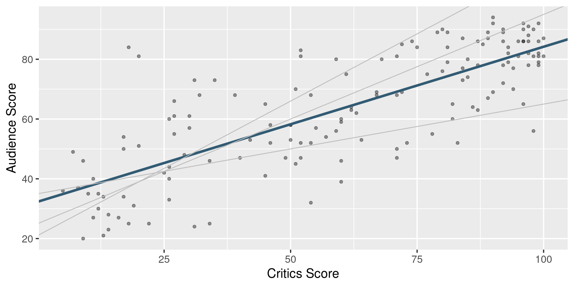
Choosing values for \(b_1\) and \(b_0\)
Residuals
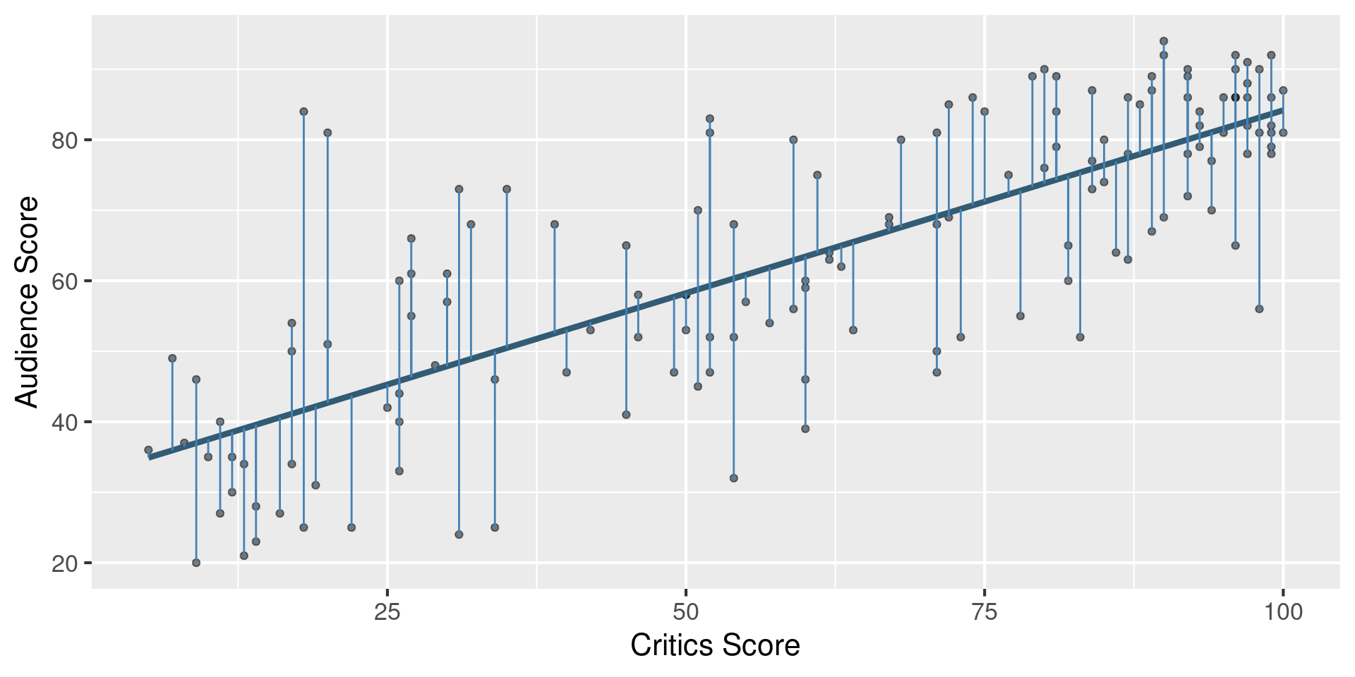
\[\text{residual} = \text{observed} - \text{predicted} = y - \hat{y}\]
Least squares line
- The residual for the \(i^{th}\) observation is
\[e_i = \text{observed} - \text{predicted} = y_i - \hat{y}_i\]
- The sum of squared residuals is
\[e^2_1 + e^2_2 + \dots + e^2_n\]
- The least squares line is the one that minimizes the sum of squared residuals
Least squares line
Slope and intercept
Properties of least squares regression
The regression line goes through the center of mass point (the coordinates corresponding to average \(X\) and average \(Y\)): \(b_0 = \bar{Y} - b_1~\bar{X}\)
Slope has the same sign as the correlation coefficient: \(b_1 = r \frac{s_Y}{s_X}\)
Sum of the residuals is zero: \(\sum_{i = 1}^n \epsilon_i = 0\)
Residuals and \(X\) values are uncorrelated
Interpreting the slope
The slope of the model for predicting audience score from critics score is 0.519. Which of the following is the best interpretation of this value?
- For every one point increase in the critics score, the audience score goes up by 0.519 points, on average.
- For every one point increase in the critics score, we expect the audience score to be higher by 0.519 points, on average.
- For every one point increase in the critics score, the audience score goes up by 0.519 points.
- For every one point increase in the audience score, the critics score goes up by 0.519 points, on average.
Interpreting slope & intercept
\[\widehat{\text{audience}} = 32.3 + 0.519 \times \text{critics}\]
- Slope: For every one point increase in the critics score, we expect the audience score to be higher by 0.519 points, on average.
- Intercept: If the critics score is 0 points, we expect the audience score to be 32.3 points.
Is the intercept meaningful?
✅ The intercept is meaningful in context of the data if
- the predictor can feasibly take values equal to or near zero or
- the predictor has values near zero in the observed data
🛑 Otherwise, it might not be meaningful!
Application exercise
Application exercise: ae-11-penguins-modeling
- Go back to your project called
ae. - If there are any uncommitted files, commit them, and push.
- Pull, and then work on
ae-11-penguins-modeling.qmd.