Quantifying uncertainty with bootstrap intervals

Lecture 20

Dr. Mine Çetinkaya-Rundel

Duke University
STA 199 - Spring 2024

2024-04-02

Warm up

While you wait for class to begin…

Any questions from prepare materials?

Announcements

• Lab 7 (last lab) is due Monday 4/8 at 8 am
• Have at least one team meeting this week to review feedback and make some progress on your lab for peer review after exam on Monday 4/15

Quantifying uncertainty

Case study: Airbnb in Asheville, NC

We have data on the price per guest (ppg) for a random sample of 50 Airbnb listings in 2020 for Asheville, NC. We are going to use these data to investigate what we would of expected to pay for an Airbnb in in Asheville, NC in June 2020.

We have data on the price per guest (ppg) for a random sample of 50 Airbnb listings in 2020 for Asheville, NC. We are going to use these data to investigate what we would of expected to pay for an Airbnb in in Asheville, NC in June 2020.

abb <- read_csv("data/asheville.csv")

glimpse(abb)

Rows: 50
Columns: 1
$ ppg <dbl> 48.00000, 40.00000, 99.00000, 13.00000, 55.00000, 75.00000, 74.00000, 169.00…

Terminology

• Population parameter - What we are interested in. Statistical measure that describes an entire population.

• Sample statistic (point estimate) - describes a sample. A piece of information you get from a fraction of the population.

abb |> 
  summarize(ppg_mean = mean(ppg))

# A tibble: 1 × 1
  ppg_mean
     <dbl>
1     76.6

Catching a fish

Suppose you’re fishing in a murky lake. Are you more likely to catch a fish using a spear or a net?

• Spear \(\rightarrow\) point estimate
• Net \(\rightarrow\) interval estimate

Constructing confidence intervals

Quantifying the variability of the sample statistics to help calculate a range of plausible values for the population parameter of interest:

• Via simulation \(\rightarrow\) using bootstrapping – using a statistical procedure that re samples a single data set to create many simulated samples.

• Via mathematical formulas \(\rightarrow\) using the Central Limit Theorem

Bootstrapping, what?

• The term bootstrapping comes from the phrase “pulling oneself up by one’s bootstraps”, which is a metaphor for accomplishing an impossible task without any outside help.

• Impossible task: estimating a population parameter using data from only the given sample.

Note

Note: This notion of saying something about a population parameter using only information from an observed sample is the crux of statistical inference, it is not limited to bootstrapping.

Bootstrapping, how?

• Resample with replacement from our data n times, where n is the sample size
• Calculate the sample statistic of interest of the new, resampled (bootstrapped) sample and record the value
• Do this entire process many many times to build the bootstrap distribution

Bootstrapping Airbnb rentals

set.seed(25) 

boot_dist_abb <- abb |>
  specify(response = ppg) |>
  generate(reps = 100, type = "bootstrap") |>
  calculate(stat = "mean")

The bootstrap distribution

glimpse(boot_dist_abb)

Rows: 100
Columns: 2
$ replicate <int> 1, 2, 3, 4, 5, 6, 7, 8, 9, 10, 11, 12, 13, 14, 15, 16, 17, 18, 19, 20,…
$ stat      <dbl> 73.11500, 78.78333, 80.19333, 83.42000, 70.15000, 73.03667, 76.41333, …

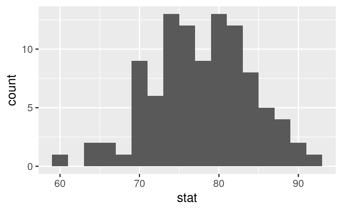
Visualzing the bootstrap distribution

What do you expect the center of the bootstrap distribution to be? Why? Check your guess by visualizing the distribution.

ggplot(boot_dist_abb, aes(x = stat)) + 
  geom_histogram(binwidth = 2)

Calculating the bootstrap distribution

boot_dist_abb |>
  summarize(
    lower = quantile(stat, 0.025),
    upper = quantile(stat, 0.975)
  )

# A tibble: 1 × 2
  lower upper
  <dbl> <dbl>
1  64.7  89.6

Interpretation

• Think
• Submit

Which of the following is the correct interpretation of the bootstrap interval?

1. There is a 95% probability the true mean price per guest for an Airbnb in Asheville is between $64.7 and $89.6.

2. There is a 95% probability the price per guest for an Airbnb in Asheville in this sample is between $64.7 and $89.6.

3. We are 95% confident the true mean price per guest for Airbnbs in Asheville is between $64.7 and $89.6.

4. We are 95% confident the price per guest for an Airbnb in Asheville in this sample is between $64.7 and $89.6.

Leveraging tidymodels tools further

Calculating the observed sample statistic:

obs_stat_abb <- abb |>
  specify(response = ppg) |>
  calculate(stat = "mean")  

Leveraging tidymodels tools further

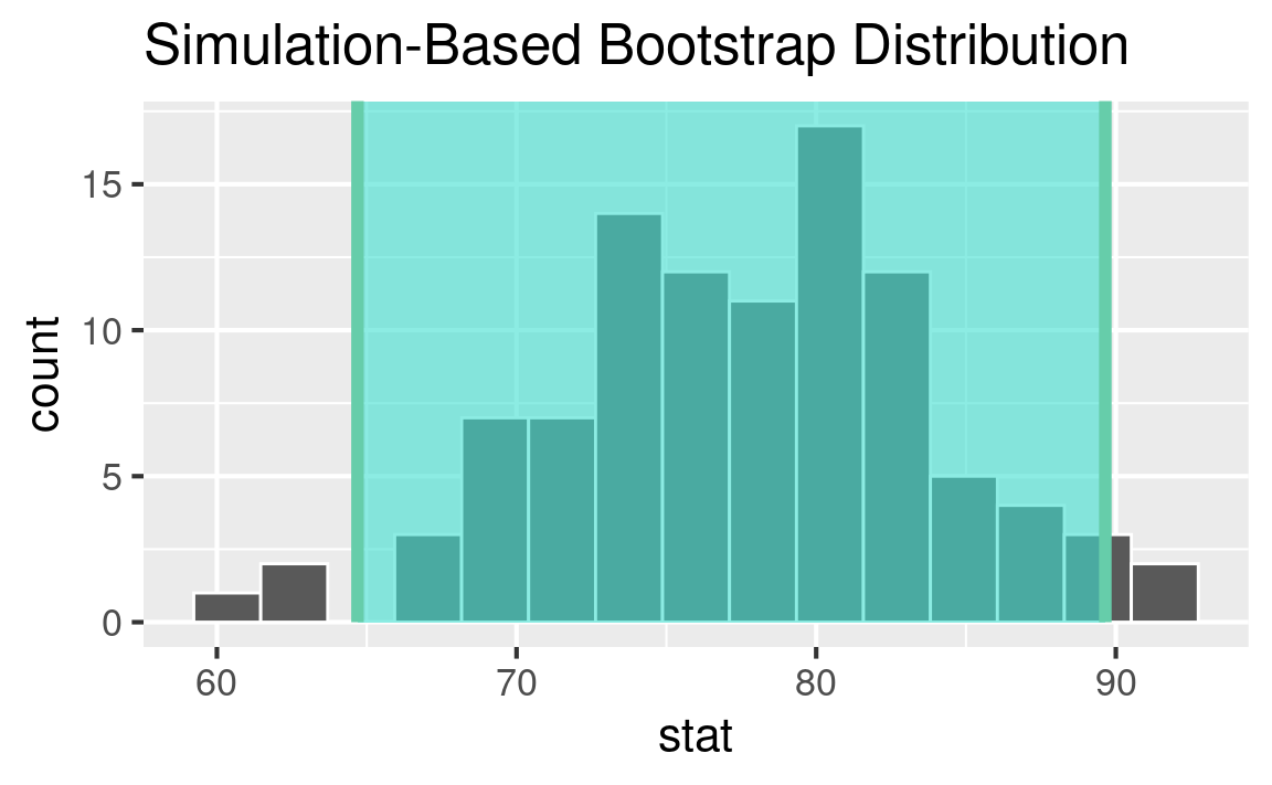
Calculating the interval:

ci_95_abb <- boot_dist_abb |>
  get_confidence_interval(
    point_estimate = obs_stat_abb, 
    level = 0.95
  )

Leveraging tidymodels tools further

Visualizing the interval:

visualize(boot_dist_abb) +
  shade_confidence_interval(ci_95_abb)

Application exercise

Application exercise: ae-15-duke-forest-bootstrap

• Go back to your project called ae.
• If there are any uncommitted files, commit them, and push.
• Work on ae-15-duke-forest-bootstrap.qmd.