Making decisions with randomization tests

Lecture 21

Dr. Mine Çetinkaya-Rundel

Duke University
STA 199 - Spring 2024

2024-04-04

Warm up

While you wait for class to begin…

• Go back to your project called ae.
• If there are any uncommitted files, commit them, and push.
• Finish working on ae-15-duke-forest-bootstrap.qmd.

Trivia

What is this visualization about?

Announcements

• Have at least one team meeting this week to review feedback and make some progress on your lab for peer review after exam on Monday 4/15

From last time: ae-15-duke-forest-bootstrap

Review last part of ae-15-duke-forest-bootstrap.qmd.

Goals

• Review constructing confidence intervals via bootstrapping
• Hypothesis testing, p-values, and making conclusions
  • Test a claim about a population parameter
  • Use simulation-based methods to generate the null distribution
  • Calculate and interpret the p-value
  • Use the p-value to draw conclusions in the context of the data and the research question

Review

Bootstrap intervals

• Why do we construct confidence intervals?
• What is bootstrapping?
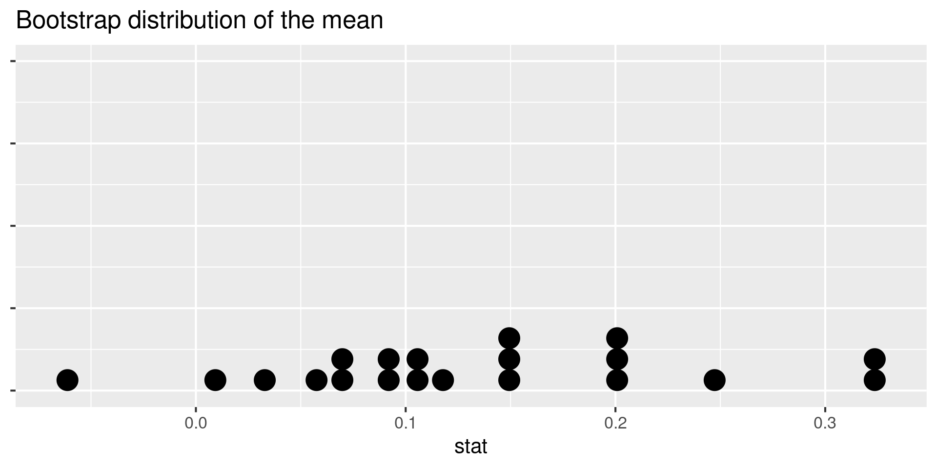
• What does each dot on the plot represent? Note: The plot is of a bootstrap distribution of a sample mean.

Why do we construct confidence intervals?

To estimate plausible values of a parameter of interest, e.g., a slope (\(\beta_1\)), a mean (\(\mu\)), a proportion (\(p\)).

What is bootstrapping?

• Bootstrapping is a statistical procedure that resamples(with replacement) a single data set to create many simulated samples.

• We then use these simulated samples to quantify the uncertainty around the sample statistic we’re interested in, e.g., a slope (\(b_1\)), a mean (\(\bar{x}\)), a proportion (\(\hat{p}\)).

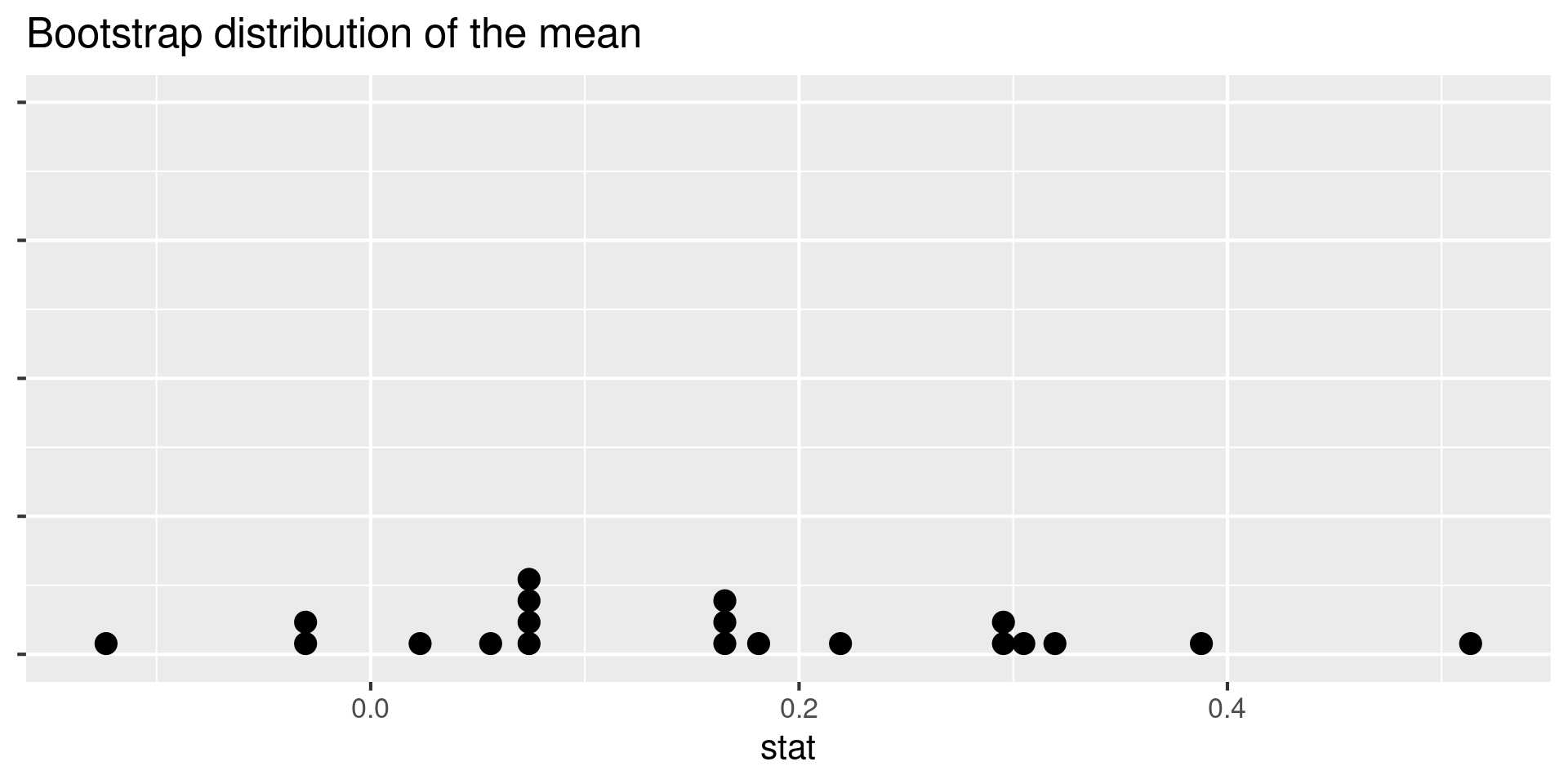
What does each dot on the plot represent?

Note: The plot is of a bootstrap distribution of a sample mean.

• Resample, with replacement, from the original data
• Do this 20 times (since there are 20 dots on the plot)
• Calculate the summary statistic of interest in each of these samples

Bootstrapping for categorical data

• specify(response = x, success = "success level")

• calculate(stat = "prop")

Bootstrapping for other stats

• calculate() documentation: infer.tidymodels.org/reference/calculate.html

• infer pipelines: infer.tidymodels.org/articles/observed_stat_examples.html

Hypothesis testing

Hypothesis testing

A hypothesis test is a statistical technique used to evaluate competing claims using data

• Null hypothesism \(H_0\): An assumption about the population. “There is nothing going on.”

• Alternative hypothesis, \(H_A\): A research question about the population. “There is something going on”.

Note: Hypotheses are always at the population level!

Writing hypotheses

As a researcher, you are interested in the average number of cups of coffee Duke students drink in a day. An article on The Chronicle suggests that the Duke students drink, on average, 1.2 cups of coffee. You are interested in evaluating if The Chronicle’s claim is too high. What are your hypotheses?

Writing hypotheses

As a researcher, you are interested in the average number of cups of coffee Duke students drink in a day.

• An article on The Chronicle suggests that the Duke students drink, on average, 1.2 cups of coffee. \(\rightarrow H_0: \mu = 1.2\)

• You are interested in evaluating if The Chronicle’s too high. \(\rightarrow H_A: \mu < 1.2\)

Collecting data

Let’s suppose you manage to take a random sample of 100 Duke students and ask them how many cups of coffee they drink and calculate the sample average to be \(\bar{x} = 1\).

Hypothesis testing “mindset”

• Assume yoi live in a world where null hypothesis is true: \(\mu = 1.2\).

• Ask yourself how likely you are to observe the sample statistic, or something even more extreme, in this world: \(P(\bar{x} < 1 | \mu = 1.2)\) = ?

  • Read: Probability that the sample mean is smaller than 1 given that the population mean is 1.2.

Application exercise

Application exercise: ae-16-equality-randomization

• Go back to your project called ae.
• If there are any uncommitted files, commit them, and push.
• Then pull and work on ae-16-equality-randomization.qmd.

Recap of AE

• A hypothesis test is a statistical technique used to evaluate competing claims (null and alternative hypotheses) using data.
• We simulate a null distribution using our original data.
• We use our sample statistic and direction of the alternative hypothesis to calculate the p-value.
• We use the p-value to determine conclusions about the alternative hypotheses.