AE 12: Modeling penguins with multiple predictors

Body mass vs. flipper length

The regression model for body mass vs. flipper length is as follows.

bm_fl_fit <- linear_reg() |>
  fit(body_mass_g ~ flipper_length_mm, data = penguins)

tidy(bm_fl_fit)

# A tibble: 2 × 5
  term              estimate std.error statistic   p.value
  <chr>                <dbl>     <dbl>     <dbl>     <dbl>
1 (Intercept)        -5781.     306.       -18.9 5.59e- 55
2 flipper_length_mm     49.7      1.52      32.7 4.37e-107

And here is the model visualized:

ggplot(penguins, aes(x = flipper_length_mm, y = body_mass_g)) +
  geom_point(alpha = 0.5) +
  geom_smooth(method = "lm")

`geom_smooth()` using formula = 'y ~ x'

Warning: Removed 2 rows containing non-finite values (`stat_smooth()`).

Warning: Removed 2 rows containing missing values (`geom_point()`).

Demo: What is the estimated body mass for a penguin with a flipper length of 210?

penguin_210 <- tibble(flipper_length_mm = 210)

predict(bm_fl_fit, new_data = penguin_210)

# A tibble: 1 × 1
  .pred
  <dbl>
1 4653.

Your turn: What is the estimated body mass for a penguin with a flipper length of 100?

But we shouldn’t do this prediction based on this model since 100 mm is outside of the range of the data (extrapolation).

penguin_100 <- tibble(flipper_length_mm = 100)

bm_fl_fit |>
  predict(new_data = penguin_100)

# A tibble: 1 × 1
  .pred
  <dbl>
1 -812.

Body mass vs. island

Demo: A different researcher wants to look at body weight of penguins based on the island they were recorded on. How are the variables involved in this analysis different?

Predictor is categorical.

Demo: Make an appropriate visualization to investigate this relationship below. Additionally, calculate the mean body mass by island.

ggplot(penguins, aes(x = island, y = body_mass_g)) +
  geom_boxplot()

Warning: Removed 2 rows containing non-finite values (`stat_boxplot()`).

penguins |>
  group_by(island) |>
  summarize(mean_bm = mean(body_mass_g, na.rm = TRUE))

# A tibble: 3 × 2
  island    mean_bm
  <fct>       <dbl>
1 Biscoe      4716.
2 Dream       3713.
3 Torgersen   3706.

Demo: Change the geom of your previous plot to geom_point(). Use this plot to think about how R models these data.

ggplot(penguins, aes(x = island, y = body_mass_g)) +
  geom_point()

Warning: Removed 2 rows containing missing values (`geom_point()`).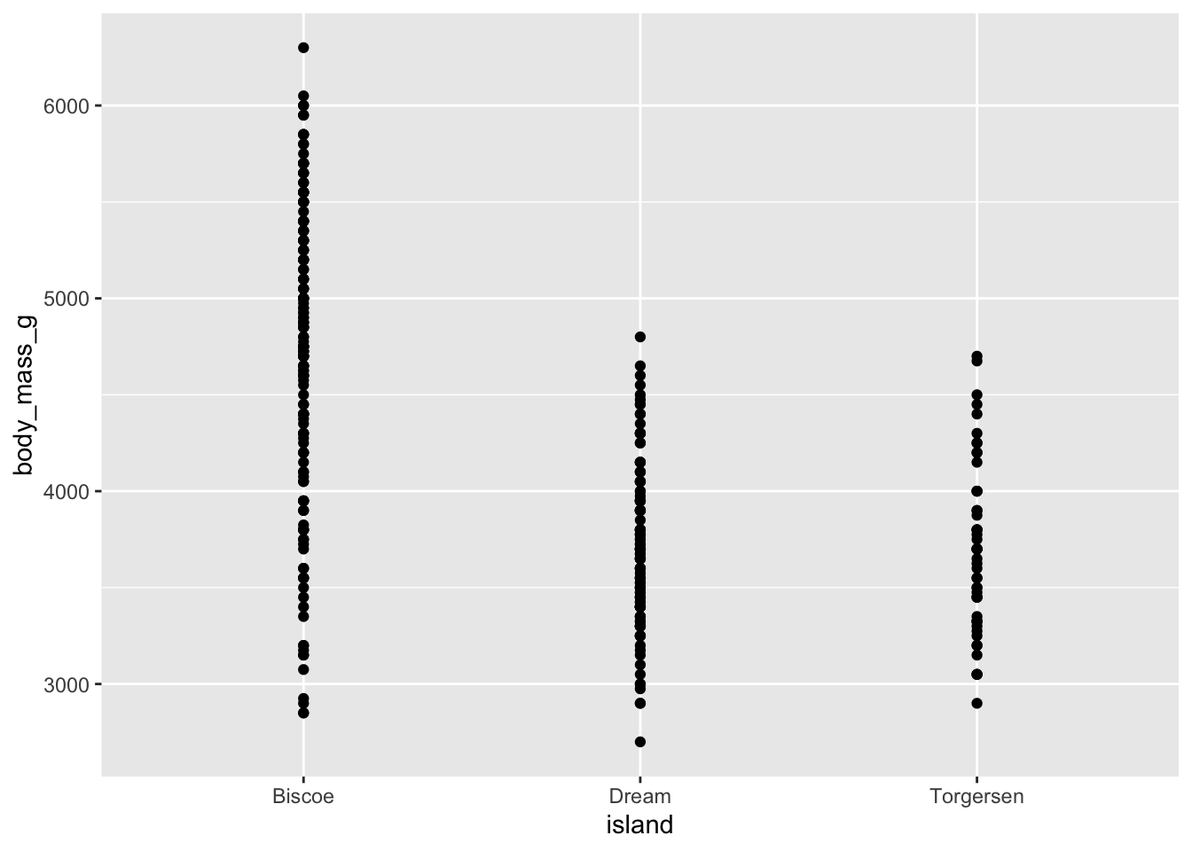

Your turn: Fit the linear regression model and display the results. Write the estimated model output below.

bm_island_fit <- linear_reg() |>
  fit(body_mass_g ~ island, data = penguins)

tidy(bm_island_fit)

# A tibble: 3 × 5
  term            estimate std.error statistic   p.value
  <chr>              <dbl>     <dbl>     <dbl>     <dbl>
1 (Intercept)        4716.      48.5      97.3 8.93e-250
2 islandDream       -1003.      74.2     -13.5 1.42e- 33
3 islandTorgersen   -1010.     100.      -10.1 4.66e- 21

Demo: Interpret each coefficient in context of the problem.
- Intercept: Penguins from Biscoe island are expected to weigh, on average, 4,716 grams.
- Slopes:
  - Penguins from Dream island are expected to weigh, on average, 1,003 grams less than those from Biscoe island.
  - Penguins from Torgersen island are expected to weigh, on average, 1,010 grams less than those from Biscoe island.
Demo: What is the estimated body weight of a penguin on Biscoe island? What are the estimated body weights of penguins on Dream and Torgersen islands?

new_penguins <- tibble(island = c("Biscoe", "Dream", "Torgersen"))

predict(bm_island_fit, new_data = new_penguins)

# A tibble: 3 × 1
  .pred
  <dbl>
1 4716.
2 3713.
3 3706.

Body mass vs. flipper length and island

Next, we will expand our understanding of models by continuing to learn about penguins. So far, we modeled body mass by flipper length, and in a separate model, modeled body mass by island. Could it be possible that the estimated body mass of a penguin changes by both their flipper length AND by the island they are on?

Demo: Fit a model to predict body mass from flipper length and island. Display the summary output and write out the estimate regression equation below.

bm_fl_island_fit <- linear_reg() |>
  fit(body_mass_g ~ flipper_length_mm + island, data = penguins)

tidy(bm_fl_island_fit)

# A tibble: 4 × 5
  term              estimate std.error statistic  p.value
  <chr>                <dbl>     <dbl>     <dbl>    <dbl>
1 (Intercept)        -4625.     392.      -11.8  4.29e-27
2 flipper_length_mm     44.5      1.87     23.9  1.65e-74
3 islandDream         -262.      55.0      -4.77 2.75e- 6
4 islandTorgersen     -185.      70.3      -2.63 8.84e- 3

\[ \widehat{body~mass} = -4625 + 44.5 \times flipper~length - 262 \times Dream - 185 \times Torgersen \]

Additive vs. interaction models

Your turn: Run the two chunks of code below and create two separate plots. How are the two plots different than each other? Which plot does the model we fit above represent?

# Plot A
ggplot(
  penguins, 
  aes(x = flipper_length_mm, y = body_mass_g, color = island)
  ) +
  geom_point(alpha = 0.5) +
  geom_smooth(method = "lm") +
  labs(title = "Plot A - Interaction model") +
  theme(legend.position = "bottom")

`geom_smooth()` using formula = 'y ~ x'

Warning: Removed 2 rows containing non-finite values (`stat_smooth()`).

Warning: Removed 2 rows containing missing values (`geom_point()`).

# Plot B
bm_fl_island_aug <- augment(bm_fl_island_fit, new_data = penguins)
ggplot(
  bm_fl_island_aug, 
  aes(x = flipper_length_mm, y = body_mass_g, color = island)
  ) +
  geom_point(alpha = 0.5) +
  geom_smooth(aes(y = .pred), method = "lm") +
  labs(title = "Plot B - Additive model") +
  theme(legend.position = "bottom")

`geom_smooth()` using formula = 'y ~ x'

Warning: Removed 2 rows containing non-finite values (`stat_smooth()`).
Removed 2 rows containing missing values (`geom_point()`).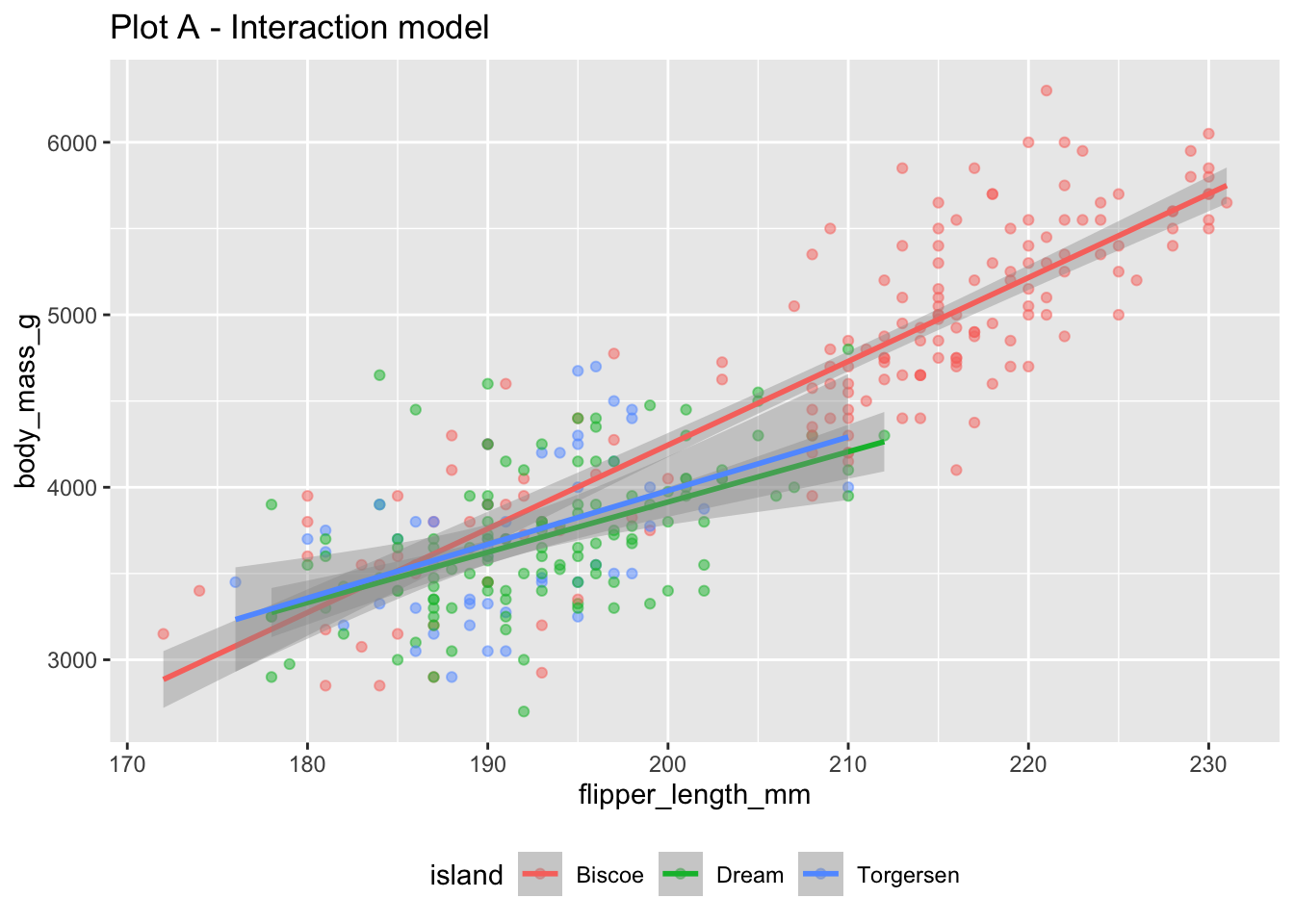

Plot B represent the model we fit.

Your turn: Interpret the slope coefficient for flipper length in the context of the data and the research question.

For every 1 millimeter the flipper is longer, we expect body mass to be higher, on average, by 44.5 grams, holding all else (the island) constant. In other words, this is true for penguins in a given island, regardless of the island.

Demo: Predict the body mass of a Dream island penguin with a flipper length of 200 mm.

penguin_200_Dream <- tibble(
  flipper_length_mm = 200,
  island = "Dream"
)

predict(bm_fl_island_fit, new_data = penguin_200_Dream)

# A tibble: 1 × 1
  .pred
  <dbl>
1 4021.

Review: Look back at Plot B. What assumption does the additive model make about the slopes between flipper length and body mass for each of the three islands?

The additive model assumes the same slope between body mass and flipper length for all three islands.

Demo: Now fit the interaction model represented in Plot A and write the estimated regression model.

bm_fl_island_int_fit <- linear_reg() |>
  fit(body_mass_g ~ flipper_length_mm * island, data = penguins)

tidy(bm_fl_island_int_fit)

# A tibble: 6 × 5
  term                              estimate std.error statistic  p.value
  <chr>                                <dbl>     <dbl>     <dbl>    <dbl>
1 (Intercept)                        -5464.     431.      -12.7  2.51e-30
2 flipper_length_mm                     48.5      2.05     23.7  1.66e-73
3 islandDream                         3551.     969.        3.66 2.89e- 4
4 islandTorgersen                     3218.    1680.        1.92 5.62e- 2
5 flipper_length_mm:islandDream        -19.4      4.94     -3.93 1.03e- 4
6 flipper_length_mm:islandTorgersen    -17.4      8.73     -1.99 4.69e- 2

\[ \widehat{body~mass} = -5464 \\ + 48.5 \times flipper~length \\ + 3551 \times Dream + 3218 \times Torgersen \\ - 19.4 \times flipper~length*Dream - 17.4 \times flipper~length*Torgersen \]

Review: What does modeling body mass with an interaction effect get us that without doing so does not?

The interaction effect allows us to model the rate of change in estimated body mass as flipper length increases as different in the three islands.

Your turn: Predict the body mass of a Dream island penguin with a flipper length of 200 mm.

predict(bm_fl_island_int_fit, new_data = penguin_200_Dream)

# A tibble: 1 × 1
  .pred
  <dbl>
1 3915.

Choosing a model

Rule of thumb: Occam’s Razor - Don’t overcomplicate the situation! We prefer the simplest best model.

glance(bm_fl_island_fit)

# A tibble: 1 × 12
  r.squared adj.r.squared sigma statistic   p.value    df logLik   AIC   BIC
      <dbl>         <dbl> <dbl>     <dbl>     <dbl> <dbl>  <dbl> <dbl> <dbl>
1     0.774         0.772  383.      386. 7.60e-109     3 -2517. 5045. 5064.
# ℹ 3 more variables: deviance <dbl>, df.residual <int>, nobs <int>

glance(bm_fl_island_int_fit)

# A tibble: 1 × 12
  r.squared adj.r.squared sigma statistic   p.value    df logLik   AIC   BIC
      <dbl>         <dbl> <dbl>     <dbl>     <dbl> <dbl>  <dbl> <dbl> <dbl>
1     0.786         0.783  374.      246. 4.55e-110     5 -2508. 5031. 5057.
# ℹ 3 more variables: deviance <dbl>, df.residual <int>, nobs <int>

Review: What is R-squared? What is adjusted R-squared?

R-squared is the percent variability in the response that is explained by our model. (Can use when models have same number of variables for model selection)

Adjusted R-squared is similar, but has a penalty for the number of variables in the model. (Should use for model selection when models have different numbers of variables).

Your turn

Now, explore body mass, and it’s relationship to bill length and flipper length. Brainstorm: How could we visualize this?
Fit the additive model. Interpret the slope for flipper in context of the data and the research question.

bm_fl_bl <- linear_reg() |>
  fit(body_mass_g ~ flipper_length_mm + bill_length_mm, data = penguins)

tidy(bm_fl_bl)

# A tibble: 3 × 5
  term              estimate std.error statistic  p.value
  <chr>                <dbl>     <dbl>     <dbl>    <dbl>
1 (Intercept)       -5737.      308.      -18.6  7.80e-54
2 flipper_length_mm    48.1       2.01     23.9  7.56e-75
3 bill_length_mm        6.05      5.18      1.17 2.44e- 1

Holding all other variables constant, for every additional millimeter in flipper length, we expect the body mass of penguins to be higher, on average, by 48.1 grams.