AE 15: Modeling houses in Duke Forest

Suggested answers

In this application exercise, we will

• use bootstrapping to quantify the uncertainty around a measure of center – median
• use bootstrapping to quantify the uncertainty around a measure of relationship – slope
• interpret confidence intervals

The dataset are on housing prices in Duke Forest – a dataset you’ve seen before! It’s called duke_forest and it’s in the openintro package. Additionally, we’ll use tidyverse and tidymodels packages.

library(tidyverse)
library(tidymodels)
library(openintro)

Typical size of a house in Duke Forest

Exercise 1

Visualize the distribution of sizes of houses in Duke Forest. What is the size of a typical house?

ggplot(duke_forest, aes(x = area)) +
  geom_histogram(binwidth = 250)

Exercise 2

Construct a 95% confidence interval for the typical size of a house in Duke Forest. Interpret the interval in context of the data.

set.seed(12345)
df_araa_median_boot <- duke_forest |>
  specify(response = area) |>
  generate(reps = 100, type = "bootstrap") |>
  calculate(stat = "median")

ggplot(df_araa_median_boot, aes(x = stat)) +
  geom_histogram(binwidth = 50)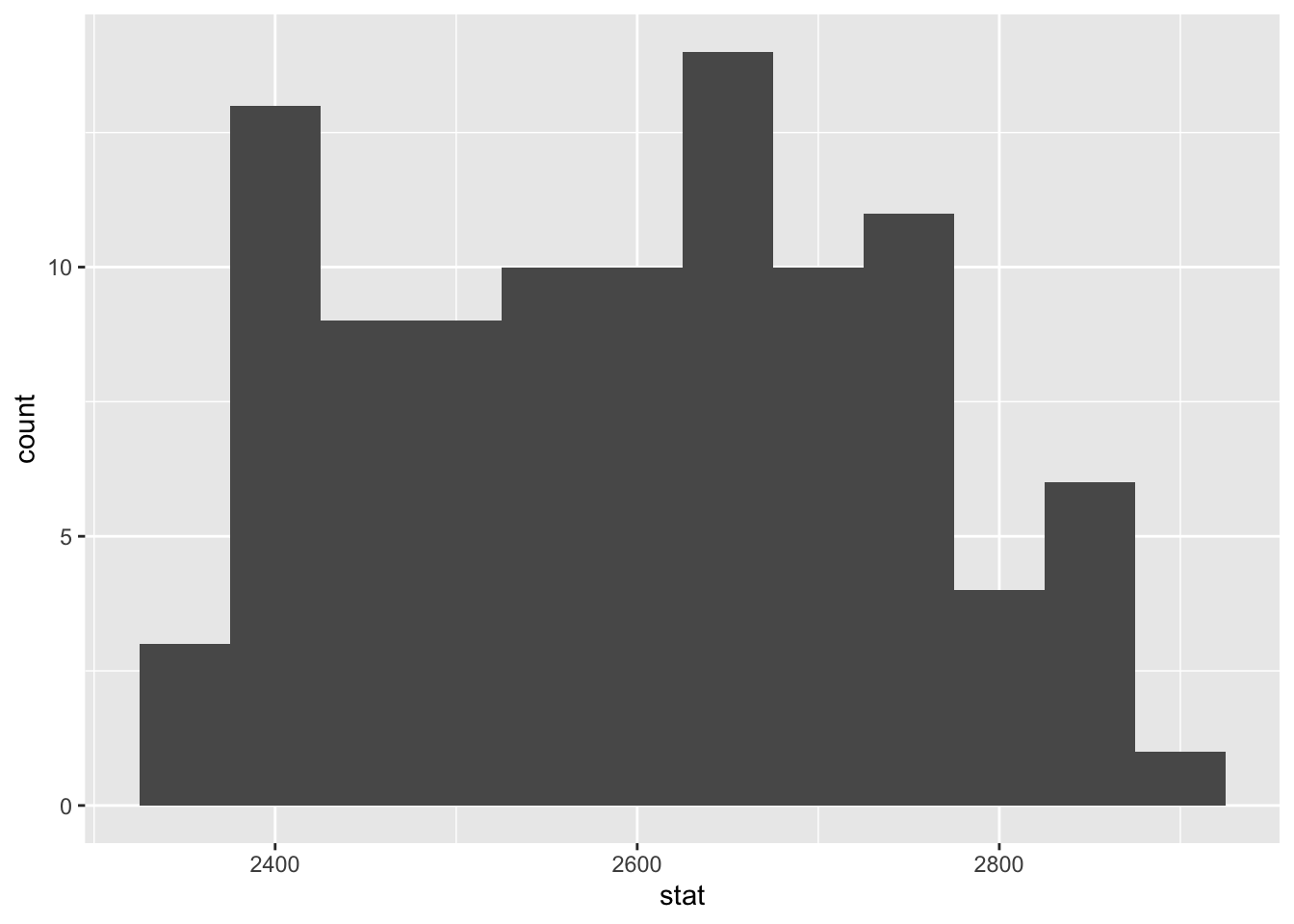

df_araa_median_boot |>
  summarize(
    l = quantile(stat, 0.025),
    u = quantile(stat, 0.975)
  )

# A tibble: 1 × 2
      l     u
  <dbl> <dbl>
1 2365. 2836.

We are 95% confident that the median house in Duke Forest is between 2,365 and 2,836 square feet.

Exercise 3

Without calculating it – would a 90% confidence interval be wider or narrower? Why?

Narrower, lower confidence level needed so we can be more precise.

Exercise 4

Construct the 90% confidence interval and interpret it.

df_araa_median_boot |>
  summarize(
    l = quantile(stat, 0.05),
    u = quantile(stat, 0.95)
  )

# A tibble: 1 × 2
      l     u
  <dbl> <dbl>
1 2395.  2830

We are 95% confident that the median house in Duke Forest is between 2,395 and 2,830 square feet.

Relationship between price and size

The following model predicts price of a house in Duke Forest from its size.

df_price_area_fit <- linear_reg() |>
  fit(price ~ area, data = duke_forest)

tidy(df_price_area_fit)

# A tibble: 2 × 5
  term        estimate std.error statistic  p.value
  <chr>          <dbl>     <dbl>     <dbl>    <dbl>
1 (Intercept)  116652.   53302.       2.19 3.11e- 2
2 area            159.      18.2      8.78 6.29e-14

The slope can be interpreted as:

For each additional square feet, the model predicts that prices of houses in Duke Forest are higher by $159, on average.

Exercise 5

Quantify the uncertainty around this slope using a 95% bootstrap confidence interval and interpret the interval in context of the data.

df_price_area_boot <- duke_forest |>
  specify(price ~ area) |>
  generate(reps = 1000, type = "bootstrap") |>
  calculate(stat = "slope")

ggplot(df_price_area_boot, aes(x = stat)) +
  geom_histogram(binwidth = 10)

df_price_area_boot |>
  summarize(
    l = quantile(stat, 0.025),
    u = quantile(stat, 0.975)
  )

# A tibble: 1 × 2
      l     u
  <dbl> <dbl>
1  89.9  214.

We are 95% confident that, for each additional square feet, the model predicts that prices of houses in Duke Forest are higher by $89.9 to $214, on average.